Customer Analysis

Let’s create a helper function.

def customer_top(metric: str, show_cnt: bool=True, ascending=False):
    """Show Top Customers by Metric"""
    cols = ['customer_unique_id', metric]
    if show_cnt:
        cols += ['orders_cnt']
    display(
        df_customers[cols]
        .sort_values(metric, ascending=ascending)
        .set_index('customer_unique_id')
        .head(10)
    )

Number of Customers

Let’s see the total number of customers.

print(f'Total customers: {df_customers.customer_unique_id.nunique():,}')

Total customers: 95,774

Let’s examine the daily distribution of customers.

pb.configure(
    df = df_sales
    , time_column = 'order_purchase_dt'
    , time_column_label = 'Date' 
    , metric = 'customer_unique_id'
    , metric_label = 'Share of Customers'
    , metric_label_for_distribution = 'Number of Customers'
    , agg_func = 'nunique'
    , norm_by='all'
    , axis_sort_order='descending'    
)

Let’s see at statistics and distribution of the metric.

pb.metric_info(freq='D')

Summary Statistics for "nunique_customer_unique_id_per_day" (Type: Integer)

Summary			Percentiles			Detailed Stats			Value Counts
Total	602 (100%)		Max	1.13k		Mean	158.57		100	8 (1%)
Missing	---		99%	361.98		Trimmed Mean (10%)	153.65		66	7 (1%)
Distinct	262 (44%)		95%	290.95		Mode	100		140	7 (1%)
Non-Duplicate	99 (16%)		75%	212.75		Range	1128		122	7 (1%)
Duplicates	340 (56%)		50%	146		IQR	113.50		182	6 (<1%)
Dup. Values	163 (27%)		25%	99.25		Std	88.15		239	6 (<1%)
Zeros	---		5%	45		MAD	80.80		131	6 (<1%)
Negative	---		1%	10.01		Kurt	23.81		108	6 (<1%)
Memory Usage	<1 Mb		Min	4		Skew	2.53		71	6 (<1%)

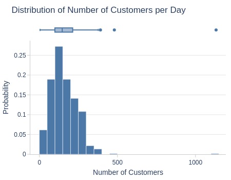
Key Observations:

• Typically 100-215 customers made purchases daily

• 5% of days had ≤45 customers, another 5% had ≥291 customers

Let’s look at the top days by the number of customers.

pb.metric_top(freq='D')

	customer_unique_id
order_purchase_dt
2017-11-24	1132
2017-11-25	480
2017-11-27	391
2017-11-26	377
2017-11-28	369
2018-08-06	368
2018-05-07	362
2018-08-07	360
2018-05-14	355
2018-05-16	350

Key Observations:

• As expected, Black Friday had the highest daily customer count

Number of Purchases

Let’s identify the top customers.

customer_top('orders_cnt', show_cnt=False)

	orders_cnt
customer_unique_id
8d50f5eadf50201ccdcedfb9e2ac8455	17
3e43e6105506432c953e165fb2acf44c	9
6469f99c1f9dfae7733b25662e7f1782	7
1b6c7548a2a1f9037c1fd3ddfed95f33	7
ca77025e7201e3b30c44b472ff346268	7
63cfc61cee11cbe306bff5857d00bfe4	6
dc813062e0fc23409cd255f7f53c7074	6
47c1a3033b8b77b3ab6e109eb4d5fdf3	6
f0e310a6839dce9de1638e0fe5ab282a	6
12f5d6e1cbf93dafd9dcc19095df0b3d	6

Key Observations:

• User ‘8d50f5eadf50201ccdcedfb9e2ac8455’ made the most purchases

Let’s see at statistics and distribution of the metric.

df_customers['orders_cnt'].explore.info(
    labels=dict(orders_cnt='Number of Orders per Customer')
    , title='Distribution of Number of Orders per Customer'
    , xaxis_type='category'
)

Summary Statistics for "orders_cnt" (Type: Integer)

Summary			Percentiles			Detailed Stats			Value Counts
Total	95.77k (100%)		Max	17		Mean	1.03		1	92.80k (97%)
Missing	---		99%	2		Trimmed Mean (10%)	1		2	2.73k (3%)
Distinct	9 (<1%)		95%	1		Mode	1		3	198 (<1%)
Non-Duplicate	2 (<1%)		75%	1		Range	16		4	30 (<1%)
Duplicates	95.77k (99%)		50%	1		IQR	0		5	8 (<1%)
Dup. Values	7 (<1%)		25%	1		Std	0.21		6	6 (<1%)
Zeros	---		5%	1		MAD	0		7	3 (<1%)
Negative	---		1%	1		Kurt	426.47		9	1 (<1%)
Memory Usage	1		Min	1		Skew	11.93		17	1 (<1%)

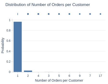
Key Observations:

• Most customers (97%) made only 1 purchase ever

• Only 3% made >1 successful purchase

Total Purchase Amount

Let’s identify the top customers.

customer_top('total_customer_payment')

	total_customer_payment	orders_cnt
customer_unique_id
0a0a92112bd4c708ca5fde585afaa872	13,664.08	1
da122df9eeddfedc1dc1f5349a1a690c	7,571.63	2
763c8b1c9c68a0229c42c9fc6f662b93	7,274.88	1
dc4802a71eae9be1dd28f5d788ceb526	6,929.31	1
459bef486812aa25204be022145caa62	6,922.21	1
ff4159b92c40ebe40454e3e6a7c35ed6	6,726.66	1
4007669dec559734d6f53e029e360987	6,081.54	1
eebb5dda148d3893cdaf5b5ca3040ccb	4,764.34	1
48e1ac109decbb87765a3eade6854098	4,681.78	1
c8460e4251689ba205045f3ea17884a1	4,655.91	4

Key Observations:

• User ‘0a0a92112bd4c708ca5fde585afaa872’ spent significantly more than others (single purchase)

Let’s see at statistics and distribution of the metric.

df_customers['total_customer_payment'].explore.info(
    labels=dict(total_customer_payment='Purchase Amount per Customer')
    , title='Distribution of Purchase Amount per Customer'
    , upper_quantile=0.99
    , hist_mode='dual_hist_trim'
)

Summary Statistics for "total_customer_payment" (Type: Float)

Summary			Percentiles			Detailed Stats			Value Counts
Total	93.23k (97%)		Max	13.66k		Mean	165.17		77.57	238 (<1%)
Missing	2.54k (3%)		99%	1.10k		Trimmed Mean (10%)	123.52		35	157 (<1%)
Distinct	28.21k (29%)		95%	469.33		Mode	77.57		73.34	147 (<1%)
Non-Duplicate	13.78k (14%)		75%	182.46		Range	13.65k		116.94	125 (<1%)
Duplicates	67.57k (71%)		50%	107.78		IQR	119.40		65	107 (<1%)
Dup. Values	14.43k (15%)		25%	63.06		Std	226.42		99.90	105 (<1%)
Zeros	---		5%	32.69		MAD	79.05		107.78	105 (<1%)
Negative	---		1%	22.75		Kurt	237.08		56.78	102 (<1%)
Memory Usage	1		Min	9.59		Skew	9.22		67.50	98 (<1%)

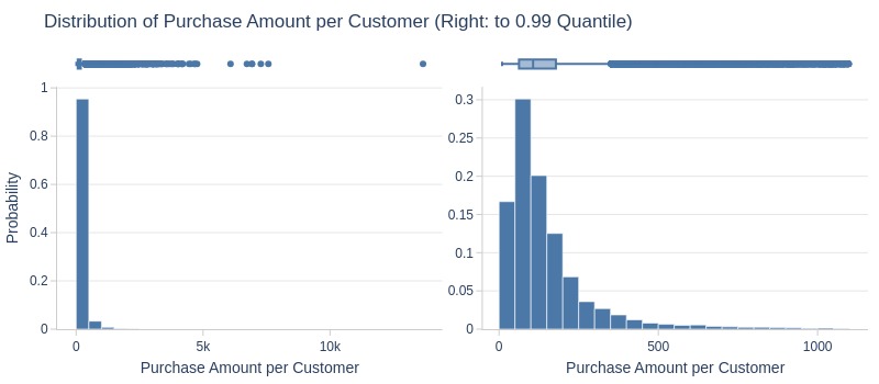
Key Observations:

• 75% of customers spent <185 R$ lifetime

• Top 5% spent ≥470 R$

Average Order Value

Let’s identify the top customers.

customer_top('avg_total_order_payment')

	avg_total_order_payment	orders_cnt
customer_unique_id
0a0a92112bd4c708ca5fde585afaa872	13,664.08	1
763c8b1c9c68a0229c42c9fc6f662b93	7,274.88	1
dc4802a71eae9be1dd28f5d788ceb526	6,929.31	1
459bef486812aa25204be022145caa62	6,922.21	1
ff4159b92c40ebe40454e3e6a7c35ed6	6,726.66	1
4007669dec559734d6f53e029e360987	6,081.54	1
eebb5dda148d3893cdaf5b5ca3040ccb	4,764.34	1
48e1ac109decbb87765a3eade6854098	4,681.78	1
edde2314c6c30e864a128ac95d6b2112	4,513.32	1
a229eba70ec1c2abef51f04987deb7a5	4,445.50	1

Key Observations:

• User ‘0a0a92112bd4c708ca5fde585afaa872’ has highest average order value (single purchase)

Let’s see at statistics and distribution of the metric.

df_customers['avg_total_order_payment'].explore.info(
    labels=dict(avg_total_order_payment='Average Order Value per Customer')
    , title='Distribution of Average Order Value per Customer'
    , upper_quantile=0.99
    , hist_mode='dual_hist_trim'
)

Summary Statistics for "avg_total_order_payment" (Type: Float)

Summary			Percentiles			Detailed Stats			Value Counts
Total	93.23k (97%)		Max	13.66k		Mean	160.29		77.57	238 (<1%)
Missing	2.54k (3%)		99%	1.06k		Trimmed Mean (10%)	120.21		35	157 (<1%)
Distinct	28.37k (30%)		95%	446.43		Mode	77.57		73.34	148 (<1%)
Non-Duplicate	14.11k (15%)		75%	176.62		Range	13.65k		116.94	125 (<1%)
Duplicates	67.40k (70%)		50%	105.65		IQR	114.25		65	107 (<1%)
Dup. Values	14.26k (15%)		25%	62.37		Std	219.68		107.78	106 (<1%)
Zeros	---		5%	32.59		MAD	76.44		99.90	105 (<1%)
Negative	---		1%	22.69		Kurt	251.54		56.78	104 (<1%)
Memory Usage	1		Min	9.59		Skew	9.42		67.50	98 (<1%)

Key Observations:

• 75% of customers have average order value <180 R$

• Top 5% have ≥445 R$

Number of Canceled Orders

Let’s identify the top customers.

customer_top('canceled_orders_cnt')

	canceled_orders_cnt	orders_cnt
customer_unique_id
46450c74a0d8c5ca9395da1daac6c120	2	3
391d6062da3dd65b4de4524f28c478de	2	2
ff36be26206fffe1eb37afd54c70e18b	2	3
6ba987d564bad1f9da8e14b9d3b71c8f	1	2
c9d0b6cc7d9fccb750ba1cc6c4b76ecb	1	1
152e41e668bcc58f2d98dcec34cc5e6f	1	1
8cfb20eff1ce8185a15ab1df1a8969e3	1	1
4fb1141f38a3efb845a83e3da0cf5278	1	1
f95ccde28c7613a61e9e40681cac6104	1	1
8028fbabf6123c13297c82f4393a4724	1	1

Key Observations:

• No user canceled >2 orders

Let’s see at statistics and distribution of the metric.

df_customers['canceled_orders_cnt'].explore.info(
    labels=dict(canceled_orders_cnt='Number of Canceled Orders')
    , title='Distribution of Number of Canceled Orders per Customer'
    , xaxis_type='category'
)

Summary Statistics for "canceled_orders_cnt" (Type: Integer)

Summary			Percentiles			Detailed Stats			Value Counts
Total	95.77k (100%)		Max	2		Mean	0.01		0	95.20k (99%)
Missing	---		99%	0		Trimmed Mean (10%)	0		1	574 (<1%)
Distinct	3 (<1%)		95%	0		Mode	0		2	3 (<1%)
Non-Duplicate	0 (<1%)		75%	0		Range	2
Duplicates	95.77k (99%)		50%	0		IQR	0
Dup. Values	3 (<1%)		25%	0		Std	0.08
Zeros	95.20k (99%)		5%	0		MAD	0
Negative	---		1%	0		Kurt	168.53
Memory Usage	1		Min	0		Skew	12.93

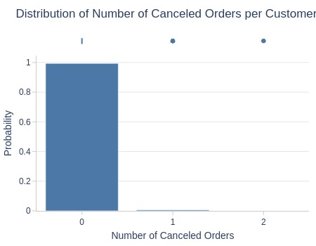
Key Observations:

• 99% of canceling users only canceled once

Canceled Order Rate

Let’s see at statistics and distribution of the metric.

df_customers['canceled_share'].explore.info(
    labels=dict(canceled_share='Share of Canceled Orders')
    , title='Distribution of Share of Canceled Orders per Customer'
    , xaxis_type='category'
)

Summary Statistics for "canceled_share" (Type: Float)

Summary			Percentiles			Detailed Stats			Value Counts
Total	95.77k (100%)		Max	1		Mean	0.01		0	95.20k (99%)
Missing	---		99%	0		Trimmed Mean (10%)	0		1	504 (<1%)
Distinct	5 (<1%)		95%	0		Mode	0		0.50	61 (<1%)
Non-Duplicate	0 (<1%)		75%	0		Range	1		0.33	10 (<1%)
Duplicates	95.77k (99%)		50%	0		IQR	0		0.67	2 (<1%)
Dup. Values	5 (<1%)		25%	0		Std	0.07
Zeros	95.20k (99%)		5%	0		MAD	0
Negative	---		1%	0		Kurt	174.22
Memory Usage	1		Min	0		Skew	13.22

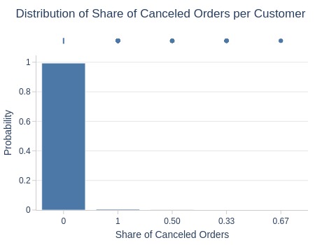
Key Observations:

• 99% of users never canceled an order

Repeat Purchase Rate

Let’s identify the top customers.

customer_top('repeat_purchase_share')

	repeat_purchase_share	orders_cnt
customer_unique_id
8d50f5eadf50201ccdcedfb9e2ac8455	0.93	17
3e43e6105506432c953e165fb2acf44c	0.89	9
1b6c7548a2a1f9037c1fd3ddfed95f33	0.86	7
ca77025e7201e3b30c44b472ff346268	0.86	7
6469f99c1f9dfae7733b25662e7f1782	0.86	7
47c1a3033b8b77b3ab6e109eb4d5fdf3	0.83	6
12f5d6e1cbf93dafd9dcc19095df0b3d	0.83	6
f0e310a6839dce9de1638e0fe5ab282a	0.83	6
63cfc61cee11cbe306bff5857d00bfe4	0.83	6
dc813062e0fc23409cd255f7f53c7074	0.83	6

Key Observations:

• User ‘8d50f5eadf50201ccdcedfb9e2ac8455’ has highest repeat purchase rate

Let’s see at statistics and distribution of the metric.

df_customers['repeat_purchase_share'].explore.info(
    labels=dict(repeat_purchase_share='Share of Repeat Purchases')
    , title='Distribution of Share of Repeat Purchases per Customer'
    , nbins=20
    , xaxis_type='category'
)

Summary Statistics for "repeat_purchase_share" (Type: Float)

Summary			Percentiles			Detailed Stats			Value Counts
Total	93.23k (97%)		Max	0.93		Mean	0.02		0	90.44k (94%)
Missing	2.54k (3%)		99%	0.50		Trimmed Mean (10%)	0		0.50	2.56k (3%)
Distinct	9 (<1%)		95%	0		Mode	0		0.67	179 (<1%)
Non-Duplicate	2 (<1%)		75%	0		Range	0.93		0.75	29 (<1%)
Duplicates	95.76k (99%)		50%	0		IQR	0		0.80	9 (<1%)
Dup. Values	7 (<1%)		25%	0		Std	0.09		0.83	5 (<1%)
Zeros	90.44k (94%)		5%	0		MAD	0		0.86	3 (<1%)
Negative	---		1%	0		Kurt	30.52		0.89	1 (<1%)
Memory Usage	1		Min	0		Skew	5.64		0.93	1 (<1%)

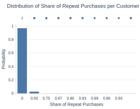
Key Observations:

• 97% of customers have no repeat purchases

Time Between Purchases

Let’s identify the top customers.

customer_top('avg_buys_diff_days')

	avg_buys_diff_days	orders_cnt
customer_unique_id
d8f3c4f441a9b59a29f977df16724f38	582.86	2
a1c61f8566347ec44ea37d22854634a1	524.10	2
a262442e3ab89611b44877c7aaf77468	521.93	2
18bc87094128bbfe943cf88adcf72059	514.51	2
7e7301841ddb4064c2f3a31e4c154932	514.28	2
24072811917876a84c81166f96aed0c1	510.90	2
408aee96c75632a92e5079eee61da399	506.27	2
97258e1c1f77f32358eccd1c9ee5954d	504.65	2
4d9e104764077f7dfae917c7cc803212	489.31	2
4658b26bcea972ed0b86a5f8c61718be	488.84	2

Key Observations:

• Many users show >500 days between purchases, but with very few purchases

• Makes average values unreliable

Let’s see at statistics and distribution of the metric.

df_customers['avg_buys_diff_days'].explore.info(
    labels=dict(avg_buys_diff_days='Average Time Between Purchases, days')
    , title='Distribution of Average Time Between Purchases'
)

Summary Statistics for "avg_buys_diff_days" (Type: Float)

Summary			Percentiles			Detailed Stats			Value Counts
Total	2.79k (3%)		Max	582.86		Mean	80.05		0.00	274 (<1%)
Missing	92.98k (97%)		99%	442.13		Trimmed Mean (10%)	58.81		0	236 (<1%)
Distinct	2.15k (2%)		95%	311.36		Mode	0.00		0.00	77 (<1%)
Non-Duplicate	2.13k (2%)		75%	124.55		Range	582.86		0.00	20 (<1%)
Duplicates	93.62k (98%)		50%	32.60		IQR	124.55		0.00	9 (<1%)
Dup. Values	19 (<1%)		25%	0.01		Std	106.09		0.00	8 (<1%)
Zeros	236 (<1%)		5%	0		MAD	48.33		0.00	6 (<1%)
Negative	---		1%	0		Kurt	2.25		0.00	5 (<1%)
Memory Usage	1		Min	0		Skew	1.63		0.00	4 (<1%)

Key Observations:

• 75% have ≤125 days between purchases

• 5% have ≥311 days

• ~30% have <1 day between purchases (likely consecutive orders)

Number of Products per Order

Let’s identify the top customers.

customer_top('avg_products_cnt')

	avg_products_cnt	orders_cnt
customer_unique_id
4546caea018ad8c692964e3382debd19	21.00	1
698e1cf81d01a3d389d96145f7fa6df8	20.00	1
c402f431464c72e27330a67f7b94d4fb	20.00	1
11f97da02237a49c8e783dfda6f50e8e	15.00	1
31e412b9fb766b6794724ed17a41dfa6	14.00	1
f7ea4eef770a388bd5b225acfc546604	14.00	1
7582a5a77fc2976628f46a13ec91b375	13.00	1
ce9f8b9c31d83341764708396ac7e38b	12.00	1
d3383e8df3cd44cd351aecff92e34627	12.00	1
37bc3d463e2a0024012a7fa587597a3c	12.00	1

Key Observations:

• Some users average 20-21 items/order (all single orders)

Let’s see at statistics and distribution of the metric.

df_customers['avg_products_cnt'].explore.info(
    labels=dict(avg_products_cnt='Average Number of Products in Order')
    , title='Distribution of Average Number of Products in Order per Customer'
    , width=600
)

Summary Statistics for "avg_products_cnt" (Type: Float)

Summary			Percentiles			Detailed Stats			Value Counts
Total	93.23k (97%)		Max	21		Mean	1.14		1	83.77k (87%)
Missing	2.54k (3%)		99%	3		Trimmed Mean (10%)	1.00		2	6.94k (7%)
Distinct	39 (<1%)		95%	2		Mode	1		3	1.18k (1%)
Non-Duplicate	8 (<1%)		75%	1		Range	20		4	444 (<1%)
Duplicates	95.73k (99%)		50%	1		IQR	0		1.50	367 (<1%)
Dup. Values	31 (<1%)		25%	1		Std	0.53		5	176 (<1%)
Zeros	---		5%	1		MAD	0		6	168 (<1%)
Negative	---		1%	1		Kurt	121.31		2.50	36 (<1%)
Memory Usage	1		Min	1		Skew	7.64		1.33	27 (<1%)

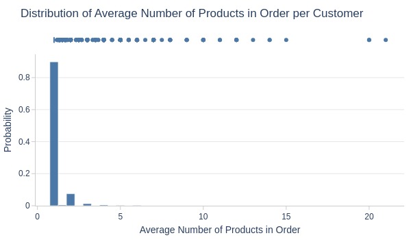
Key Observations:

• 87% average 1 item/order

• ~1% average ≥3 items

Product Price per Order

Let’s identify the top customers.

customer_top('avg_products_price')

	avg_products_price	orders_cnt
customer_unique_id
dc4802a71eae9be1dd28f5d788ceb526	6,735.00	1
459bef486812aa25204be022145caa62	6,729.00	1
ff4159b92c40ebe40454e3e6a7c35ed6	6,499.00	1
eebb5dda148d3893cdaf5b5ca3040ccb	4,690.00	1
48e1ac109decbb87765a3eade6854098	4,590.00	1
edde2314c6c30e864a128ac95d6b2112	4,399.87	1
fa562ef24d41361e476e748681810e1e	4,099.99	1
ca27f3dac28fb1063faddd424c9d95fa	4,059.00	1
011875f0176909c5cf0b14a9138bb691	3,999.90	1
edf81e1f3070b9dac83ec83dacdbb9bc	3,999.00	1

Let’s see at statistics and distribution of the metric.

df_customers['avg_products_price'].explore.info(
    labels=dict(avg_products_price='Average Product Price in Order')
    , title='Distribution of Average Product Price in Order per Customer'
    , nbins=20
)

Summary Statistics for "avg_products_price" (Type: Float)

Summary			Percentiles			Detailed Stats			Value Counts
Total	93.23k (97%)		Max	6.74k		Mean	125.87		59.90	1.85k (2%)
Missing	2.54k (3%)		99%	899.99		Trimmed Mean (10%)	90.82		69.90	1.60k (2%)
Distinct	7.96k (8%)		95%	367.63		Mode	59.90		49.90	1.50k (2%)
Non-Duplicate	4.31k (5%)		75%	139.90		Range	6.73k		89.90	1.22k (1%)
Duplicates	87.81k (92%)		50%	79		IQR	97		99.90	1.17k (1%)
Dup. Values	3.65k (4%)		25%	42.90		Std	190.66		39.90	994 (1%)
Zeros	---		5%	18.90		MAD	63.90		29.90	982 (1%)
Negative	---		1%	11.49		Kurt	117.58		79.90	981 (1%)
Memory Usage	1		Min	0.85		Skew	7.83		19.90	941 (<1%)

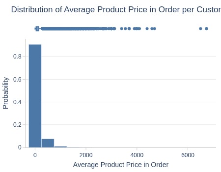
Key Observations:

• 75% have average product price ≤140 R$

• Top 5% have ≥367 R$

Number of Reviews

Let’s identify the top customers.

customer_top('reviews_cnt')

	reviews_cnt	orders_cnt
customer_unique_id
8d50f5eadf50201ccdcedfb9e2ac8455	15.00	17
3e43e6105506432c953e165fb2acf44c	9.00	9
b4e4f24de1e8725b74e4a1f4975116ed	7.00	5
ca77025e7201e3b30c44b472ff346268	7.00	7
47c1a3033b8b77b3ab6e109eb4d5fdf3	7.00	6
1b6c7548a2a1f9037c1fd3ddfed95f33	7.00	7
6469f99c1f9dfae7733b25662e7f1782	7.00	7
f0e310a6839dce9de1638e0fe5ab282a	6.00	6
12f5d6e1cbf93dafd9dcc19095df0b3d	6.00	6
35ecdf6858edc6427223b64804cf028e	6.00	5

Key Observations:

• User with id ‘8d50f5eadf50201ccdcedfb9e2ac8455’ left significantly more reviews than other users. But they also made many orders.

Let’s see at statistics and distribution of the metric.

df_customers['reviews_cnt'].explore.info(
    labels=dict(reviews_cnt='Number of Reviews per Customer')
    , title='Distribution of Number of Reviews per Customer'
    , nbins=20
)

Summary Statistics for "reviews_cnt" (Type: Integer)

Summary			Percentiles			Detailed Stats			Value Counts
Total	93.23k (97%)		Max	15		Mean	1.04		1	90.35k (94%)
Missing	2.54k (3%)		99%	2		Trimmed Mean (10%)	1		2	2.35k (2%)
Distinct	9 (<1%)		95%	1		Mode	1		3	369 (<1%)
Non-Duplicate	2 (<1%)		75%	1		Range	14		4	118 (<1%)
Duplicates	95.76k (99%)		50%	1		IQR	0		5	23 (<1%)
Dup. Values	7 (<1%)		25%	1		Std	0.25		6	11 (<1%)
Zeros	---		5%	1		MAD	0		7	5 (<1%)
Negative	---		1%	1		Kurt	208.46		9	1 (<1%)
Memory Usage	1		Min	1		Skew	10.27		15	1 (<1%)

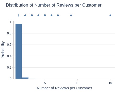
Key Observations:

• 94% left only 1 review

• 2% left 2 reviews

Review Score

Let’s identify the top customers.

customer_top('customer_avg_reviews_score')

	customer_avg_reviews_score	orders_cnt
customer_unique_id
84732c5050c01db9b23e19ba39899398	5.00	1
6c093de8084a2a18102ff996fe31bd93	5.00	1
188b92d12c9004c4087ea4d115aba44f	5.00	1
9387a3940cc2d07a9ec8b85d82fad721	5.00	1
32bd15f649096a45270727aa50df8460	5.00	1
d2cdc1bc229c5e1848f8f7ce60a415f7	5.00	1
3277ec319b5ae6c2baff32baeb1c2bf9	5.00	1
0e922f6fc526a5e89ae5b96df681a792	5.00	1
6a1829a8f4b92d3b96896ef58e522b12	5.00	1
25325d558a8e0d36fcd5e3b6a8b80eb6	5.00	1

Let’s see at statistics and distribution of the metric.

df_customers['customer_avg_reviews_score'].explore.info(
    labels=dict(customer_avg_reviews_score='Average Review Score per Customer')
    , title='Distribution of Average Review Score per Customer'
    , nbins=5
)

Summary Statistics for "customer_avg_reviews_score" (Type: Float)

Summary			Percentiles			Detailed Stats			Value Counts
Total	93.23k (97%)		Max	5		Mean	4.14		5	54.39k (57%)
Missing	2.54k (3%)		99%	5		Trimmed Mean (10%)	4.42		4	18.22k (19%)
Distinct	26 (<1%)		95%	5		Mode	5		1	9.29k (10%)
Non-Duplicate	6 (<1%)		75%	5		Range	4		3	7.78k (8%)
Duplicates	95.75k (99%)		50%	5		IQR	1		2	2.91k (3%)
Dup. Values	20 (<1%)		25%	4		Std	1.29		4.50	297 (<1%)
Zeros	---		5%	1		MAD	0		3.50	156 (<1%)
Negative	---		1%	1		Kurt	0.85		2.50	79 (<1%)
Memory Usage	1		Min	1		Skew	-1.45		1.50	23 (<1%)

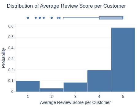
Key Observations:

• 57% average 5-star reviews

• 19% average 4-star

Delivery Cost

Let’s identify the top customers.

customer_top('avg_order_total_freight_value')

	avg_order_total_freight_value	orders_cnt
customer_unique_id
fff5eb4918b2bf4b2da476788d42051c	1,794.96	1
066ee6b9c6fc284260ff9a1274a82ca7	1,002.29	1
ef7361e14a64f77990f58e9c571e2f9a	711.33	1
fffcf5a5ff07b0908bd4e2dbc735a684	497.42	1
527f7f3237fb1397c459701bc765b6f0	497.08	1
eae0a83d752b1dd32697e0e7b4221656	480.64	2
6d394722d5fc5e721aee6875a218d8db	479.28	1
6411590d91c48640cb07e72fbb4a359e	458.73	1
f9172a6495d46451776be8bc8e46032d	456.47	1
3895f60f6e6a89e5cfb7b72ffdcdf7e0	436.24	1

Key Observations:

• User ‘fff5eb4918b2bf4b2da476788d42051c’ has unusually high shipping costs (single purchase)

Let’s see at statistics and distribution of the metric.

df_customers['avg_order_total_freight_value'].explore.info(
    labels=dict(avg_order_total_freight_value='Average Freight Value ')
    , title='Distribution of Average Freight Value per Customer'
    , upper_quantile=0.99
    , hist_mode='dual_hist_trim'
)

Summary Statistics for "avg_order_total_freight_value" (Type: Float)

Summary			Percentiles			Detailed Stats			Value Counts
Total	93.23k (97%)		Max	1.79k		Mean	22.78		15.10	2.71k (3%)
Missing	2.54k (3%)		99%	103.50		Trimmed Mean (10%)	19.06		7.78	1.67k (2%)
Distinct	8.98k (9%)		95%	54.59		Mode	15.10		14.10	1.41k (1%)
Non-Duplicate	3.81k (4%)		75%	24.10		Range	1.79k		11.85	1.33k (1%)
Duplicates	86.80k (91%)		50%	17.24		IQR	10.23		18.23	1.15k (1%)
Dup. Values	5.16k (5%)		25%	13.87		Std	21.47		7.39	1.07k (1%)
Zeros	330 (<1%)		5%	7.89		MAD	6.60		15.23	777 (<1%)
Negative	---		1%	7.39		Kurt	609.04		16.11	721 (<1%)
Memory Usage	1		Min	0		Skew	12.48		8.72	685 (<1%)

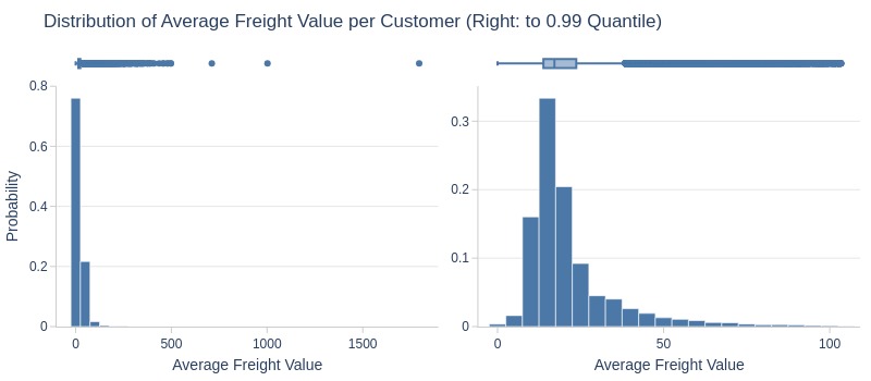
Key Observations:

• 75% have average shipping ≤24 R$

• Top 5% have ≥54 R$

Delivery Time

Let’s identify the top customers.

customer_top('avg_delivery_time_days')

	avg_delivery_time_days	orders_cnt
customer_unique_id
4a2519b6991378f6f2ce5ed22d308f03	209.63	1
eb21169c3153a2b507fc7e76d561ff14	208.35	1
f0785d41d416fa827f24c4b95d066b69	195.63	1
c6c0b794d3e4eb69cd85d1438a0db26e	194.85	1
3c2564d42f7ddd8b7576f0dd9cb1b4c5	194.63	1
4df2d7257a7463e2d7a98a5b08cb92fc	194.05	1
4cb8ad9a4554099db7d70c13d0dae906	191.46	1
78d26ae26b5bb9cb398edc7384d3c15f	189.86	1
186a453a38d349c487ccbf472b31fb39	188.13	1
e7834c7e017fb854ac65189a66c33132	187.74	1

Let’s see at statistics and distribution of the metric.

df_customers['avg_delivery_time_days'].explore.info(
    labels=dict(avg_delivery_time_days='Distribution of Average Delivery Time, days')
    , title='Distribution of Average Delivery Time'
    , upper_quantile=0.99
    , hist_mode='dual_hist_trim'
)

Summary Statistics for "avg_delivery_time_days" (Type: Float)

Summary			Percentiles			Detailed Stats			Value Counts
Total	93.10k (97%)		Max	209.63		Mean	12.55		7.09	3 (<1%)
Missing	2.67k (3%)		99%	45.90		Trimmed Mean (10%)	11.15		6.20	3 (<1%)
Distinct	90.70k (95%)		95%	29.19		Mode	Multiple		9.00	3 (<1%)
Non-Duplicate	88.34k (92%)		75%	15.68		Range	209.10		6.07	3 (<1%)
Duplicates	5.07k (5%)		50%	10.22		IQR	8.90		10.07	3 (<1%)
Dup. Values	2.35k (2%)		25%	6.78		Std	9.53		12.34	3 (<1%)
Zeros	---		5%	3.03		MAD	6.13		2.07	3 (<1%)
Negative	---		1%	1.83		Kurt	40.74		13.15	3 (<1%)
Memory Usage	1		Min	0.53		Skew	3.91		5.88	3 (<1%)

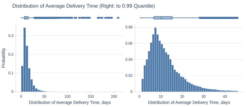
Key Observations:

• 75% have average delivery ≤16 days

• Top 5% have ≥29 days

Delivery Delay Time

Let’s identify the top customers.

customer_top('avg_delivery_delay_days')

	avg_delivery_delay_days	orders_cnt
customer_unique_id
eb21169c3153a2b507fc7e76d561ff14	188.98	1
4a2519b6991378f6f2ce5ed22d308f03	181.61	1
4cb8ad9a4554099db7d70c13d0dae906	175.87	1
78d26ae26b5bb9cb398edc7384d3c15f	167.71	1
3c2564d42f7ddd8b7576f0dd9cb1b4c5	166.58	1
f0785d41d416fa827f24c4b95d066b69	165.63	1
e7834c7e017fb854ac65189a66c33132	162.72	1
beba456e33133cc65b481399d051b2ba	161.78	1
4df2d7257a7463e2d7a98a5b08cb92fc	161.61	1
186a453a38d349c487ccbf472b31fb39	159.61	1

Let’s see at statistics and distribution of the metric.

df_customers['avg_delivery_delay_days'].explore.info(
    labels=dict(avg_delivery_delay_days='Average Delivery Delay Time, days')
    , title='Distribution of Average Delivery Delay Time'
    , lower_quantile=0.01
    , upper_quantile=0.99
    , hist_mode='dual_hist_trim'
)

Summary Statistics for "avg_delivery_delay_days" (Type: Float)

Summary			Percentiles			Detailed Stats			Value Counts
Total	93.10k (97%)		Max	188.98		Mean	-11.08		-12.39	5 (<1%)
Missing	2.67k (3%)		99%	18.85		Trimmed Mean (10%)	-11.44		-14.44	4 (<1%)
Distinct	89.02k (93%)		95%	3.81		Mode	-12.39		-13.26	4 (<1%)
Non-Duplicate	85.19k (89%)		75%	-6.38		Range	334.99		-13.28	4 (<1%)
Duplicates	6.75k (7%)		50%	-11.61		IQR	9.82		-13.29	4 (<1%)
Dup. Values	3.83k (4%)		25%	-16.21		Std	10.05		-8.19	4 (<1%)
Zeros	---		5%	-25.29		MAD	6.98		-13.17	4 (<1%)
Negative	85.56k (89%)		1%	-34.21		Kurt	30.06		-7.22	4 (<1%)
Memory Usage	1		Min	-146.02		Skew	2.22		-7.20	4 (<1%)

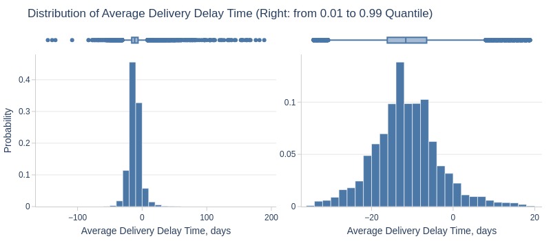
Key Observations:

• Top 5% have ≥25 days early delivery

• Median: 6-16 days early

• Bottom 5% have ≥4 days late

Order Weight

Let’s identify the top customers.

customer_top('avg_order_total_weight_kg')

	avg_order_total_weight_kg	orders_cnt
customer_unique_id
3d47f4368ccc8e1bb4c4a12dbda7111b	184.40	1
066ee6b9c6fc284260ff9a1274a82ca7	154.20	1
f0d3389b217aa61b5a66744ddd694cc3	144.30	1
6d394722d5fc5e721aee6875a218d8db	129.34	1
fff5eb4918b2bf4b2da476788d42051c	112.20	1
559026a1299bd2ede976c8d516d92258	108.50	1
96e91c0dba30f7ff60c9acd47677c248	98.40	1
38a4f1deb45ca914dd13c73b41775d71	97.00	1
fb98136edc2c0f996bfad36a0c7e1306	96.80	1
064fb6f70338688d1372235d95d92ff7	93.90	1

Let’s see at statistics and distribution of the metric.

df_customers['avg_order_total_weight_kg'].explore.info(
    labels=dict(avg_order_total_weight_kg='Average Order Weight per Customer')
    , title='Distribution of Average Order Weight per Customer'
    , upper_quantile=0.99
    , hist_mode='dual_hist_trim'    
)

Summary Statistics for "avg_order_total_weight_kg" (Type: Float)

Summary			Percentiles			Detailed Stats			Value Counts
Total	93.23k (97%)		Max	184.40		Mean	2.39		0.20	5.04k (5%)
Missing	2.54k (3%)		99%	22.35		Trimmed Mean (10%)	1.31		0.15	3.96k (4%)
Distinct	2.15k (2%)		95%	10.48		Mode	0.20		0.25	3.51k (4%)
Non-Duplicate	846 (<1%)		75%	2.10		Range	184.40		0.30	3.49k (4%)
Duplicates	93.62k (98%)		50%	0.75		IQR	1.80		0.40	3.13k (3%)
Dup. Values	1.30k (1%)		25%	0.30		Std	4.75		0.10	2.68k (3%)
Zeros	5 (<1%)		5%	0.15		MAD	0.82		0.35	2.62k (3%)
Negative	---		1%	0.10		Kurt	99.02		0.50	2.26k (2%)
Memory Usage	1		Min	0		Skew	6.64		0.60	2.16k (2%)

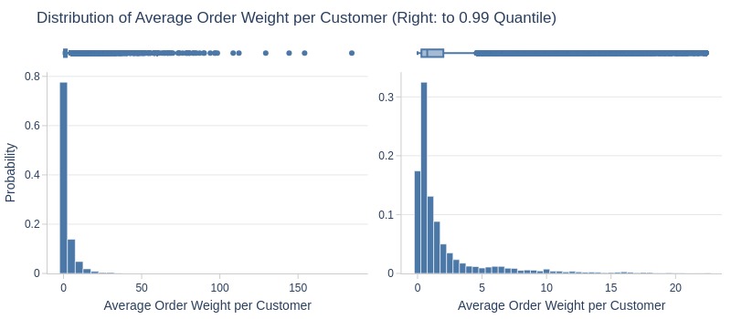
Key Observations:

• 75% have average order weight ≤2kg

• Top 5% have ≥10kg

Time from First to Second Purchase

Let’s identify the top customers.

customer_top('from_first_to_second_days')

	from_first_to_second_days	orders_cnt
customer_unique_id
d8f3c4f441a9b59a29f977df16724f38	582.86	2
a1c61f8566347ec44ea37d22854634a1	524.10	2
a262442e3ab89611b44877c7aaf77468	521.93	2
18bc87094128bbfe943cf88adcf72059	514.51	2
7e7301841ddb4064c2f3a31e4c154932	514.28	2
24072811917876a84c81166f96aed0c1	510.90	2
408aee96c75632a92e5079eee61da399	506.27	2
97258e1c1f77f32358eccd1c9ee5954d	504.65	2
e53fd5575f1418397aae732c5755b6fc	490.70	3
4d9e104764077f7dfae917c7cc803212	489.31	2

Key Observations:

• User ‘d8f3c4f441a9b59a29f977df16724f38’ has longest 1st→2nd purchase gap

customer_top('from_first_to_second_days', ascending=True)

	from_first_to_second_days	orders_cnt
customer_unique_id
3a649b3c6b379a427fa6f4a5f646a43d	0.00	2
0710e0c85fe7cb494d624e0863782e46	0.00	2
d927267e54f07b9e0fd408d2f840024c	0.00	2
c0118e2c0a037c31aeca71d0b81f66a1	0.00	3
271d3cdd872021b1b6669ad93e8b856b	0.00	2
75a2adfe9f86d401f24b5fe2eb9a582c	0.00	2
64a5301ff6bdaf1baa00058672402d7a	0.00	2
cfe96f24bd8c36325e0d92e44324cf66	0.00	2
897ecc46977d723a6e514f3ebe92c844	0.00	2
5c5a99e5ef172fbf5fc8a68e6bb2e0ab	0.00	2

Key Observations:

• Some customers made 1st/2nd purchases within seconds

Let’s see at statistics and distribution of the metric.

df_customers['from_first_to_second_days'].explore.info(
    labels=dict(from_first_to_second_days='Time From First to Second Purchase, days')
    , title='Distribution of Time From First to Second Purchase'
)

Summary Statistics for "from_first_to_second_days" (Type: Float)

Summary			Percentiles			Detailed Stats			Value Counts
Total	2.79k (3%)		Max	582.86		Mean	80.24		0.00	296 (<1%)
Missing	92.98k (97%)		99%	443.75		Trimmed Mean (10%)	58.48		0	253 (<1%)
Distinct	2.11k (2%)		95%	318.98		Mode	0.00		0.00	82 (<1%)
Non-Duplicate	2.09k (2%)		75%	125.49		Range	582.86		0.00	23 (<1%)
Duplicates	93.66k (98%)		50%	28.91		IQR	125.49		0.00	9 (<1%)
Dup. Values	18 (<1%)		25%	0.00		Std	108.08		0.00	7 (<1%)
Zeros	253 (<1%)		5%	0		MAD	42.87		0.00	5 (<1%)
Negative	---		1%	0		Kurt	2.07		0.00	4 (<1%)
Memory Usage	1		Min	0		Skew	1.60		0.00	3 (<1%)

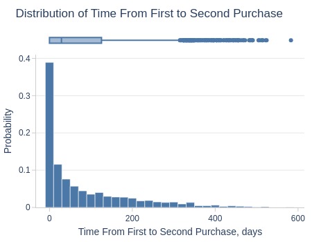
Key Observations:

• ~50% have >29 days between 1st/2nd purchase

• Top 25% have ≥125 days

• Top 5% have ≥319 days

Time from First to Last Purchase

Let’s identify the top customers.

customer_top('from_first_to_last_days')

	from_first_to_last_days	orders_cnt
customer_unique_id
d8f3c4f441a9b59a29f977df16724f38	582.86	2
8f6ce2295bdbec03cd50e34b4bd7ba0a	537.39	3
a1c61f8566347ec44ea37d22854634a1	524.10	2
a262442e3ab89611b44877c7aaf77468	521.93	2
18bc87094128bbfe943cf88adcf72059	514.51	2
7e7301841ddb4064c2f3a31e4c154932	514.28	2
1b6e96ed99cb8d135efe220d761bbd67	511.49	3
24072811917876a84c81166f96aed0c1	510.90	2
408aee96c75632a92e5079eee61da399	506.27	2
97258e1c1f77f32358eccd1c9ee5954d	504.65	2

Key Observations:

• User ‘d8f3c4f441a9b59a29f977df16724f38’ has longest 1st→last purchase span (2 purchases)

Let’s see at statistics and distribution of the metric.

df_customers['from_first_to_last_days'].explore.info(
    labels=dict(from_first_to_last_days='Time From First to Last Purchase, days')
    , title='Distribution of Time From First to Last Purchase'
)

Summary Statistics for "from_first_to_last_days" (Type: Float)

Summary			Percentiles			Detailed Stats			Value Counts
Total	2.79k (3%)		Max	582.86		Mean	87.25		0.00	281 (<1%)
Missing	92.98k (97%)		99%	448.81		Trimmed Mean (10%)	65.23		0	236 (<1%)
Distinct	2.15k (2%)		95%	334.65		Mode	0.00		0.00	77 (<1%)
Non-Duplicate	2.13k (2%)		75%	140.11		Range	582.86		0.00	21 (<1%)
Duplicates	93.62k (98%)		50%	34.83		IQR	140.10		0.00	10 (<1%)
Dup. Values	18 (<1%)		25%	0.01		Std	113.39		0.00	6 (<1%)
Zeros	236 (<1%)		5%	0		MAD	51.63		0.00	6 (<1%)
Negative	---		1%	0		Kurt	1.58		0.00	4 (<1%)
Memory Usage	1		Min	0		Skew	1.49		0.00	3 (<1%)

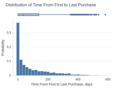
Key Observations:

• ~50% have >35 days between 1st/2nd purchase

• Top 25% have ≥140 days

• Top 5% have ≥335 days

Number of Months with Purchases

Let’s identify the top customers.

customer_top('months_with_buys')

	months_with_buys	orders_cnt
customer_unique_id
8d50f5eadf50201ccdcedfb9e2ac8455	9.00	17
ca77025e7201e3b30c44b472ff346268	6.00	7
f0e310a6839dce9de1638e0fe5ab282a	6.00	6
6469f99c1f9dfae7733b25662e7f1782	6.00	7
63cfc61cee11cbe306bff5857d00bfe4	5.00	6
7305430719d715992b00be82af4a6aa8	4.00	4
dc813062e0fc23409cd255f7f53c7074	4.00	6
a1874c5550d2f0bc14cc122164603713	4.00	4
5e8f38a9a1c023f3db718edcf926a2db	4.00	5
738ffcf1017b584e9d2684b36e07469c	4.00	4

Key Observations:

• User ‘8d50f5eadf50201ccdcedfb9e2ac8455’ had most months with purchases

Let’s see at statistics and distribution of the metric.

df_customers['months_with_buys'].explore.info(
    labels=dict(months_with_buys='Number of Months with Purchases')
    , title='Distribution of Number of Months with Purchases per Customer'
    , nbins=10 
)

Summary Statistics for "months_with_buys" (Type: Integer)

Summary			Percentiles			Detailed Stats			Value Counts
Total	93.23k (97%)		Max	9		Mean	1.02		1	91.55k (96%)
Missing	2.54k (3%)		99%	2		Trimmed Mean (10%)	1		2	1.58k (2%)
Distinct	7 (<1%)		95%	1		Mode	1		3	87 (<1%)
Non-Duplicate	2 (<1%)		75%	1		Range	8		4	17 (<1%)
Duplicates	95.77k (99%)		50%	1		IQR	0		6	3 (<1%)
Dup. Values	5 (<1%)		25%	1		Std	0.15		5	1 (<1%)
Zeros	---		5%	1		MAD	0		9	1 (<1%)
Negative	---		1%	1		Kurt	195.89
Memory Usage	1		Min	1		Skew	10.54

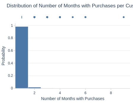
Key Observations:

• 96% of customers only purchased in 1 month

Maximum Consecutive Months with Purchases

Let’s identify the top customers.

customer_top('max_consecutive_months_with_buys')

	max_consecutive_months_with_buys	orders_cnt
customer_unique_id
8d50f5eadf50201ccdcedfb9e2ac8455	6.00	17
6469f99c1f9dfae7733b25662e7f1782	5.00	7
1b6c7548a2a1f9037c1fd3ddfed95f33	4.00	7
3e43e6105506432c953e165fb2acf44c	3.00	9
e0836a97eaae86ac4adc26fbb334a527	3.00	3
e0c99ffdcd8891130985ac90cd2d8eec	3.00	3
f0e310a6839dce9de1638e0fe5ab282a	3.00	6
935b9c5a3162185f88dac06d8d08d623	3.00	3
2ddc001b620bd90d0f4378cfde1db887	3.00	4
ca77025e7201e3b30c44b472ff346268	3.00	7

Let’s see at statistics and distribution of the metric.

df_customers['max_consecutive_months_with_buys'].explore.info(
    labels=dict(max_consecutive_months_with_buys='Maximum Consecutive Months with Purchases')
    , title='Distribution of Maximum Consecutive Months with Purchases'
    , nbins=10 
)

Summary Statistics for "max_consecutive_months_with_buys" (Type: Integer)

Summary			Percentiles			Detailed Stats			Value Counts
Total	93.23k (97%)		Max	6		Mean	1.00		1	92.79k (97%)
Missing	2.54k (3%)		99%	1		Trimmed Mean (10%)	1		2	438 (<1%)
Distinct	6 (<1%)		95%	1		Mode	1		3	8 (<1%)
Non-Duplicate	3 (<1%)		75%	1		Range	5		4	1 (<1%)
Duplicates	95.77k (99%)		50%	1		IQR	0		6	1 (<1%)
Dup. Values	3 (<1%)		25%	1		Std	0.07		5	1 (<1%)
Zeros	---		5%	1		MAD	0
Negative	---		1%	1		Kurt	523.67
Memory Usage	1		Min	1		Skew	18.41

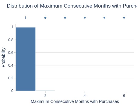
Key Observations:

• Maximum consecutive months: 6 (1 customer)

• 3 consecutive months: 8 customers

• 2 consecutive months: 438 customers

Additional Metrics

• What percentage of customers make only one purchase?

tmp_df_res = df_sales.groupby(['customer_unique_id'])['order_id'].nunique()

display(f'{(tmp_df_res[tmp_df_res == 1].count() * 100 / tmp_df_res.count()).round(2)}% of customers make a purchase only once')

'97.01% of customers make a purchase only once'

• What percentage of customers make more than one purchase?

display(f'{(tmp_df_res[tmp_df_res > 1].count() * 100 / tmp_df_res.count()).round(2)}% of customers make more than one purchase')

'2.99% of customers make more than one purchase'

• What percentage of customers make more than two purchases?

display(f'{(tmp_df_res[tmp_df_res > 2].count() * 100 / tmp_df_res.count()).round(2)}% of customers make more than two purchases')

'0.24% of customers make more than two purchases'

• What percentage of customers make more than three purchases?

display(f'{(tmp_df_res[tmp_df_res > 3].count() * 100 / tmp_df_res.count()).round(2)}% of customers make more than two purchases')

'0.05% of customers make more than two purchases'

• What percentage of customers make 4 or more purchases?

for n in range(4, 10):
    display(f'{(tmp_df_res[tmp_df_res > n].count() * 100 / tmp_df_res.count()).round(2)}% of customers make more than {n} two purchases')

'0.02% of customers make more than 4 two purchases'

'0.01% of customers make more than 5 two purchases'

'0.01% of customers make more than 6 two purchases'

'0.0% of customers make more than 7 two purchases'

'0.0% of customers make more than 8 two purchases'

'0.0% of customers make more than 9 two purchases'

• Are there customers who make purchases regularly (monthly)?

tmp_df_res = df_sales[['order_purchase_dt', 'customer_unique_id', 'order_id']].dropna(subset='order_purchase_dt')
tmp_df_res['year_month'] = tmp_df_res.order_purchase_dt.dt.to_period('M')
tmp_df_res['first_month'] = tmp_df_res.groupby('customer_unique_id')['year_month'].transform('min')
last_month = tmp_df_res['year_month'].max()

tmp_df_res = (tmp_df_res.groupby('customer_unique_id', as_index=False)
          .agg(
              year_months = ('year_month', 'nunique')
              , first_month = ('first_month', 'first')              
          )
)
tmp_df_res['all_months'] = (last_month - tmp_df_res.first_month).apply(lambda x: x.n + 1)
tmp_df_res['is_in_all_months'] = tmp_df_res['all_months'] == tmp_df_res['year_months']
tmp_df_res = tmp_df_res[tmp_df_res.is_in_all_months]

tmp_df_res.sort_values('all_months', ascending=False).head(10)

	customer_unique_id	year_months	first_month	all_months	is_in_all_months
81877	e0836a97eaae86ac4adc26fbb334a527	3	2018-06	3	True
23908	4186b96df8197e7b4982a751c1dde3b6	2	2018-07	2	True
9611	1a2ede4e787ad199c46719ecb02d81ea	2	2018-07	2	True
75435	cef42836ff25476d55c9a3e58f8da99d	2	2018-07	2	True
5194	0e381ce773b382849206115413009851	2	2018-07	2	True
31177	5568fb2b583235812ed08eb9587d0465	2	2018-07	2	True
42598	74b8021516f25eb91f5b4e704a2cd671	2	2018-07	2	True
33646	5c00e849b56a56ea31560d5d66f933e9	2	2018-07	2	True
77501	d44f553a3663a6323c901cf1f0a47c87	2	2018-07	2	True
45360	7c588c097689b0b77fd73d171332b0ba	2	2018-07	2	True

Key Observations:

• No customers purchased in all months

• Maximum regular purchases: 2 consecutive months