Slice Analysis

Black Friday

Let’s examine Black Friday, specifically November 24, 2017.

We will consider November 23-25 to account for one day before and one day after.

mask = df_orders.order_purchase_dt.between('2017-11-23', '2017-11-26')
df_black_orders = df_orders[mask]
mask = df_sales.order_purchase_dt.between('2017-11-23', '2017-11-26')
df_black_sales = df_sales[mask]

Number of Sales

By Hour

pb.configure(
    df = df_black_sales
    , time_column = 'order_purchase_dt'
    , time_column_label = 'Date'
    , metric = 'order_id'
    , metric_label = 'Number of Sales'
    , agg_func = 'nunique'
    , freq = 'h'
)
pb.line_resample()

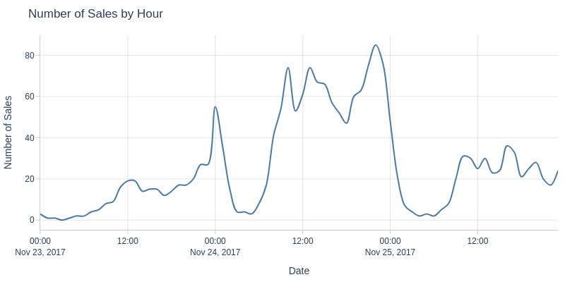
Key Observations:

• Sales grew from 5AM-10AM (first peak)

• Second peak at 1PM

• Decline until 6PM

• Evening growth until 10PM peak

• Anomalous spike at midnight Nov 24 (Black Friday start)

pb.configure(
    df = df_black_sales
    , time_column = 'order_purchase_dt'
    , time_column_label = 'Date'
    , metric = 'order_id'
    , metric_label = 'Share of Sales'
    , agg_func = 'nunique'
    , freq = 'h'
    , norm_by='all'
    , axis_sort_order='descending'    
    , text_auto='.1%'
    , update_fig={'xaxis': {'tickformat': '.0%'}}
)

By Payment Category

pb.bar_groupby(y='order_total_payment_cat', to_slide='_black_friday')

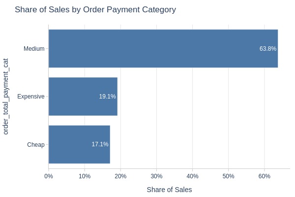
Key Observations:

• 64% of orders are medium-priced

By Order Weight Category

pb.bar_groupby(y='order_total_weight_cat', to_slide='_black_friday')

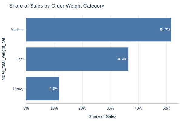
Key Observations:

• 52% medium weight, 36% light

By Delivery Time Category

pb.bar_groupby(y='delivery_time_days_cat', to_slide='_black_friday')

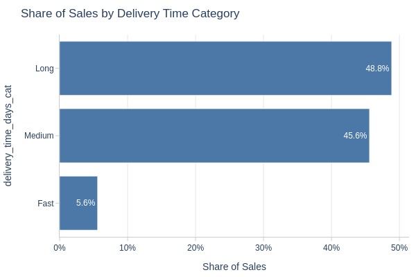
Key Observations:

• Delivery time categories:

  • Long: 49%

  • Medium: 46%

  • Fast: 6%

• Black Friday increased delivery times

By Presence of Installment Payments

pb.bar_groupby(y='order_has_installment', to_slide='_black_friday')

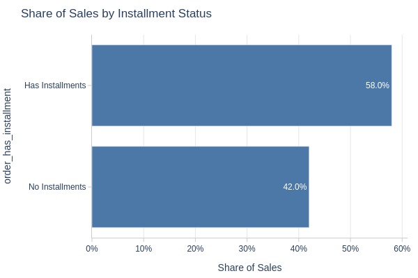
Key Observations:

• 58% of orders used installments

By Payment Type

pb.bar_groupby(y='order_payment_types', to_slide='_black_friday')

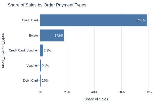
Key Observations:

• Payment methods:

  • Credit card: 79%

  • Boleto: 18%

By Product Category

pb.bar_groupby(
    y='order_product_categories'
    , to_slide='_black_friday'
)

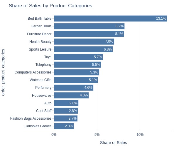
Key Observations:

• The majority of orders consisted of products from the Bed Bath Table category (13%).

By Generalized Product Category

pb.bar_groupby(y='order_general_product_categories', to_slide='_black_friday')

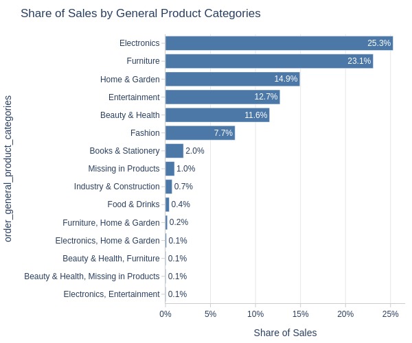
Key Observations:

• Top generalized categories:

  • Bed Bath Table: 25%

  • Furniture: 23%

By Review Score

pb.bar_groupby(y='order_avg_reviews_score', to_slide='_black_friday')

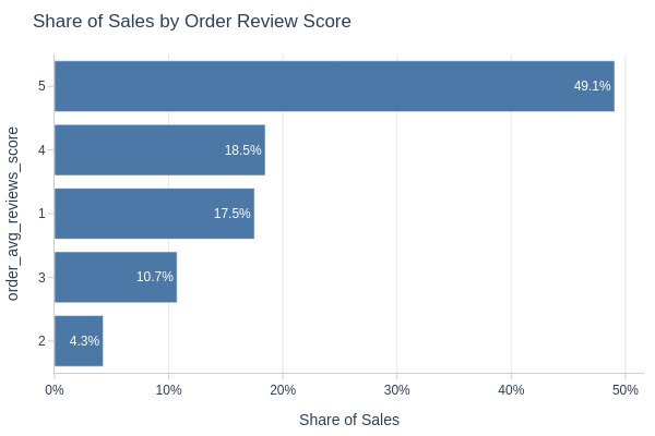
Key Observations:

• Review scores:

  • 5 stars: 49%

  • 1 star: 17.5%

  • 3 stars: 10.7%

  • 2 stars: 4.3%

By Top Customer States

pb.bar_groupby(y='customer_state', to_slide='_black_friday')

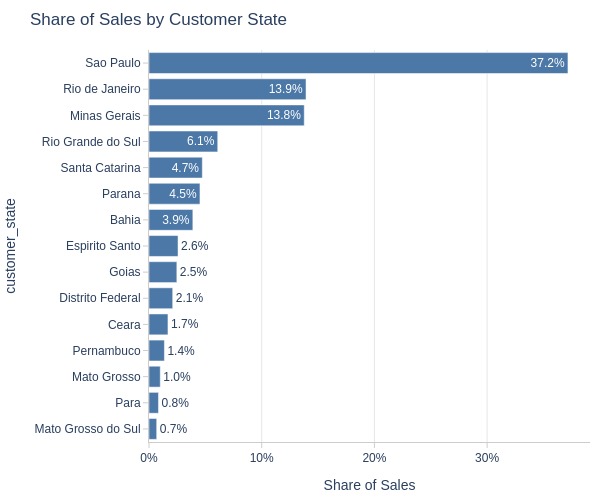
Key Observations:

• Sales by state:

  • São Paulo: 37%

  • Rio/Minas: 14% each

  • Others: ≤6%

By Top Customer Cities

pb.bar_groupby(y='customer_city', to_slide='_black_friday')

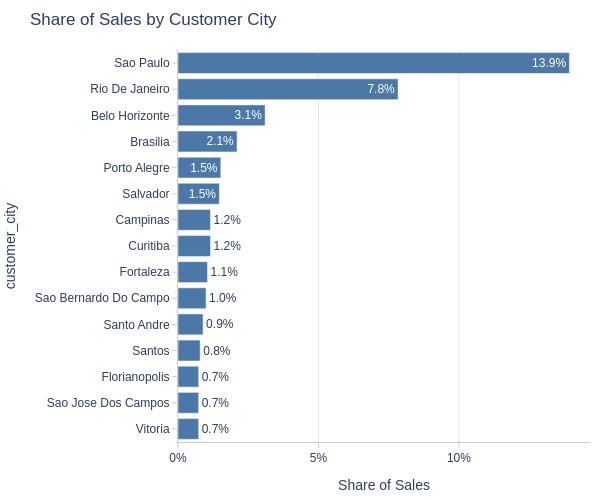
Key Observations:

• Sales by city:

  • São Paulo: 14%

  • Rio: 8%

  • Others: ≤3%

Sum of Sales

By Hour

pb.configure(
    df = df_black_sales
    , time_column = 'order_purchase_dt'
    , time_column_label = 'Date'
    , metric = 'total_payment'
    , metric_label = 'Sales Amount, R$'
    , title_base = 'Sales Amount'
    , agg_func = 'sum'
    , freq = 'h'
)
pb.line_resample(to_slide='_black_friday')

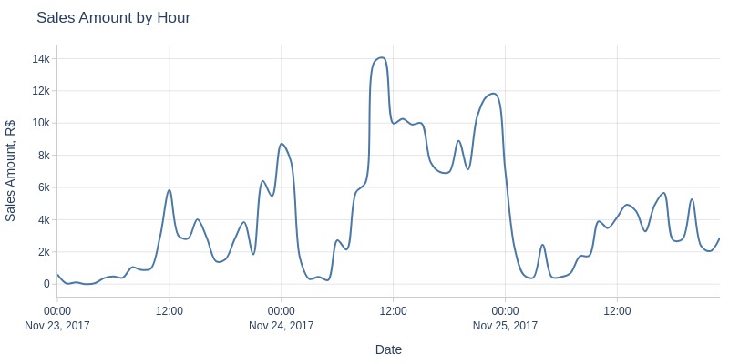
Key Observations:

• Revenue peaked 10-11AM, declined until 6PM, then rose without surpassing morning peak

Average Order Value

By Hour

pb.configure(
    df = df_black_sales
    , time_column = 'order_purchase_dt'
    , time_column_label = 'Date'
    , metric = 'total_payment'
    , metric_label = 'Average Order Value, R$'
    , metric_label_for_distribution = 'Order Value, R$'
    , title_base = 'Average Order Value'
    , agg_func = 'mean'
    , freq='h'
)
pb.line_resample(to_slide='_black_friday')

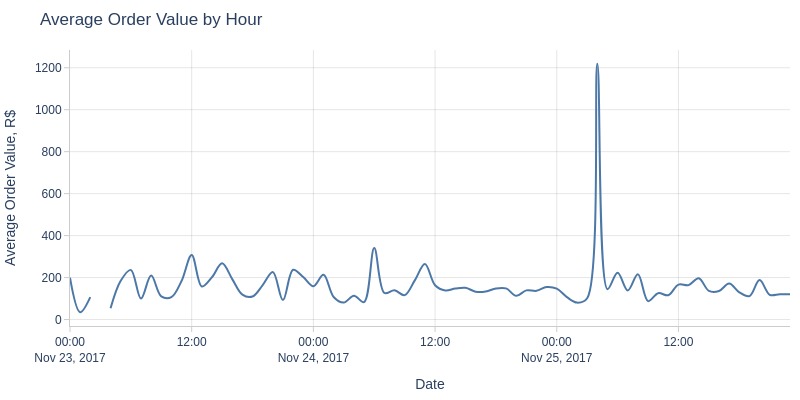
Key Observations:

• There is an anomalous hour (4 AM) on November 25, 2017, in the average order value.

• It is not clear that the average order value was higher on Black Friday compared to the neighboring days.

pb.configure(
    df = df_black_sales
    , metric = 'total_payment'
    , metric_label = 'Average Order Value, R$'
    , metric_label_for_distribution = 'Order Value, R$'
    , agg_func = 'mean'
    , title_base = 'Average Order Value and Number of Sales'
    , axis_sort_order='descending'
    , text_auto='.0f'
)

Top Orders.

pb.metric_top()

	total_payment
order_id
2cc9089445046817a7539d90805e6e5a	6,081.54
27db1a079a22bec1453d0f24f630005f	2,429.68
acf01c9262ddb5d9adae8daa34e31568	2,416.00
7eb6bfea5daf19a607f08fd25ea7672a	2,106.55
a123264c1f8bef4f19be2d4245017920	1,798.01
c9dff4871bed0bc5d4b917767a22d67d	1,740.39
404ae63d165e7de5dd0bade9787b50c0	1,425.56
6ddfbf514959b49b6410c01ad93054bb	1,359.40
3b6bf8d07e34c52b0f65c58afb3df15b	1,334.28
2a1f2a555014d3eb75492fd0a08942a1	1,274.51

Let’s see at statistics and distribution of the metric.

pb.metric_info(
    labels=dict(total_payment='Order Value, R$')
    , title='Distribution of Order Value'
    , upper_quantile=0.95
    , hist_mode='dual_hist_trim'
)

Summary Statistics for "total_payment" (Type: Float)

Summary			Percentiles			Detailed Stats			Value Counts
Total	1.90k (100%)		Max	6.08k		Mean	155.46		66.67	37 (2%)
Missing	---		99%	957.54		Trimmed Mean (10%)	116.09		66.64	22 (1%)
Distinct	1.38k (73%)		95%	427.99		Mode	66.67		62.44	14 (<1%)
Non-Duplicate	1.12k (59%)		75%	168.90		Range	6.07k		62.41	11 (<1%)
Duplicates	523 (27%)		50%	99.78		IQR	106.89		39.60	8 (<1%)
Dup. Values	256 (13%)		25%	62.01		Std	230.49		168.36	7 (<1%)
Zeros	---		5%	33.84		MAD	70.10		116.94	7 (<1%)
Negative	---		1%	23.78		Kurt	246.85		117.85	7 (<1%)
Memory Usage	<1 Mb		Min	13.78		Skew	11.68		30	7 (<1%)

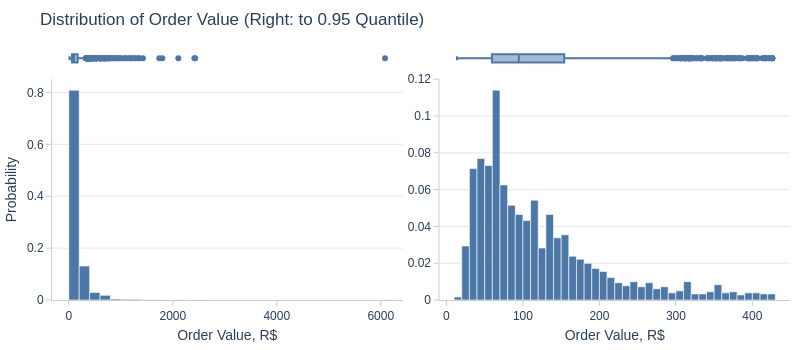
Key Observations:

• 75% of Black Friday orders ≤170 R\( (many >1000 R\) outliers)

By Top Customer States

pb.bar_groupby(
    y='customer_state'
    , show_count=True
).show()

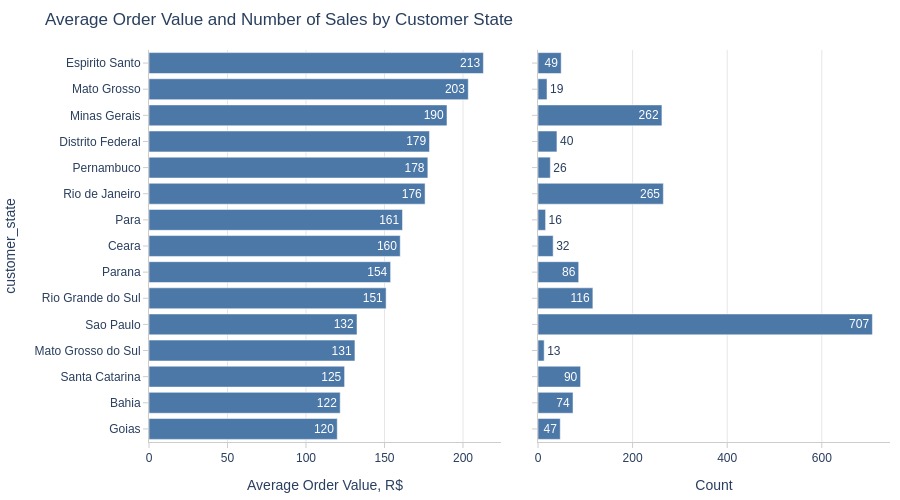
Key Observations:

• Highest order values in:

  1. Espírito Santo

  2. Mato Grosso

  3. Minas Gerais

Number of Customers

By Hour

pb.configure(
    df = df_black_sales
    , time_column = 'order_purchase_dt'
    , time_column_label = 'Date'
    , metric = 'customer_unique_id'
    , metric_label = 'Number of Customers'
    , agg_func = 'nunique'
    , freq = 'h'
)
pb.line_resample(to_slide='_black_friday')

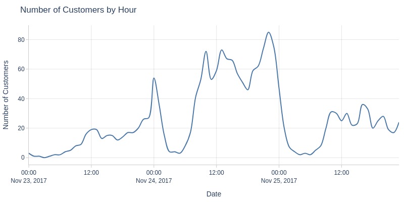
Key Observations:

• Customer count trend matches order count (mostly single orders)

There is no sense in looking at it by segments, as customers primarily made only one order, and the results would be similar to the order count.

Share of Unavailable Orders

pb.configure(
    time_column = 'order_purchase_dt'
    , time_column_label = 'Date'
    , metric = 'target_share'
    , metric_label = 'Share of Unavailable Orders'
    , freq='ME'
)

tmp_tmp_df_res = df_black_orders['order_status'].preproc.calc_target_category_share(
    target_category='Unavailable'
    , group_columns=['order_purchase_dt']
    , resample_freq = 'h'
)

pb.line(
    data_frame=tmp_tmp_df_res
)

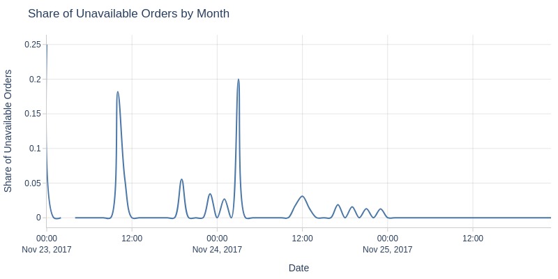
Key Observations:

• The proportion of orders with the status unavailable has spikes at 0 AM and 10 AM on November 23, 2017, and at 3 AM on November 24, 2017. There is also a very strong spike on November 26, 2017.

• It is not clear that there was a shortage of products specifically on Black Friday.

Reviews Score

pb.configure(
    df = df_black_sales
    , metric = 'order_avg_reviews_score'
    , metric_label = 'Average Order Reviews Score'
    , metric_label_for_distribution = 'Order Reviews Score'
)

pb.metric_info(
    labels=dict(order_avg_reviews_score='Order Reviews Score')
    , title='Distribution of Order Reviews Score'
    , xaxis_type='category'
)

Summary Statistics for "order_avg_reviews_score" (Type: Integer)

Summary			Percentiles			Detailed Stats			Value Counts
Total	1.90k (100%)		Max	5		Mean	3.77		5	933 (49%)
Missing	---		99%	5		Trimmed Mean (10%)	3.97		4	351 (18%)
Distinct	5 (<1%)		95%	5		Mode	5		1	333 (18%)
Non-Duplicate	0 (<1%)		75%	5		Range	4		3	204 (11%)
Duplicates	1.90k (99%)		50%	4		IQR	2		2	81 (4%)
Dup. Values	5 (<1%)		25%	3		Std	1.51
Zeros	---		5%	1		MAD	1.48
Negative	---		1%	1		Kurt	-0.73
Memory Usage	<1 Mb		Min	1		Skew	-0.90

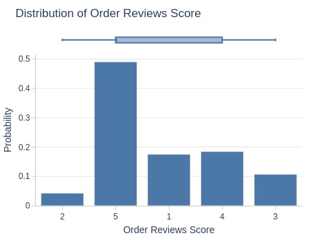
Key Observations:

• 49% of Nov 23-25 orders had 5-star reviews

Canceled Orders

Analyze canceled orders.

df_canceled = df_orders[df_orders.order_status=='Canceled']

Number of Orders

By month

pb.configure(
    df = df_canceled
    , time_column = 'order_purchase_dt'
    , time_column_label = 'Date'
    , metric = 'order_id'
    , metric_label = 'Number of Canceled Orders'
    , agg_func = 'nunique'
    , freq = 'ME'
)
pb.line_resample()

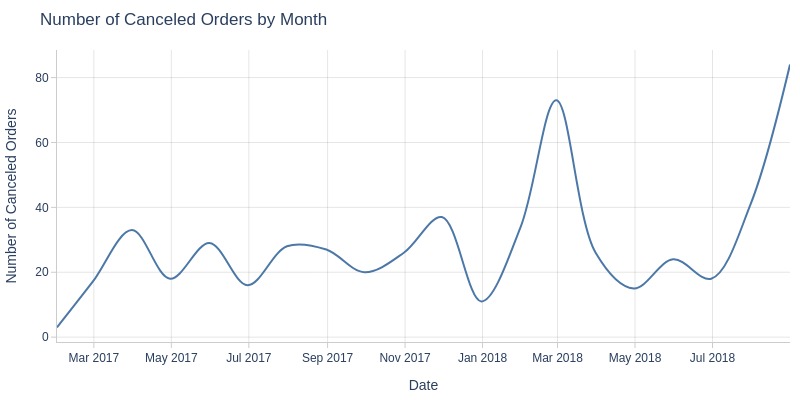
Key Observations:

• Typically 20-40 canceled orders/month

• Anomalous spikes in Feb/Aug 2018

pb.configure(
    df = df_canceled
    , time_column = 'order_purchase_dt'
    , time_column_label = 'Date'
    , metric = 'order_id'
    , metric_label = 'Share of Canceled Orders'
    , agg_func = 'nunique'
    , freq = 'h'
    , norm_by='all'
    , axis_sort_order='descending'    
    , text_auto='.1%'
    , update_fig={'xaxis': {'tickformat': '.0%'}}
)

By Payment Category

pb.bar_groupby(y='order_total_payment_cat')

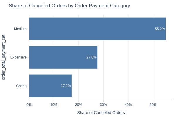
Key Observations:

• Canceled orders:

  • Medium price: 55%

  • Expensive: 28%

By Order Weight Category

pb.bar_groupby(y='order_total_weight_cat')

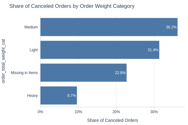
Key Observations:

• Canceled order weights:

  • Medium: 36%

  • Light: 31%

By Presence of Installment Payments

pb.bar_groupby(y='order_has_installment')

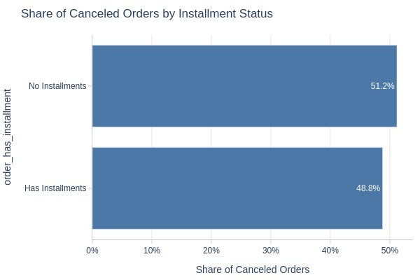
Key Observations:

• 51% of canceled orders didn’t use installments

By Payment Type

pb.bar_groupby(y='order_payment_types')

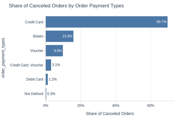
Key Observations:

• Canceled order payments:

  • Credit card: 70%

  • Boleto: 16%

  • Voucher: 10% (higher than overall)

By Product Category

pb.bar_groupby(
    y='order_product_categories'
    , text_auto=False
)

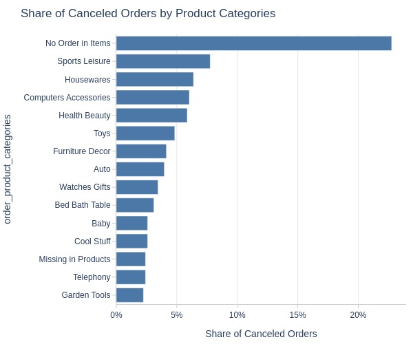
Key Observations:

• Top canceled order categories:

  1. Bed Bath Table

  2. Health Beauty

  3. Sports Leisure

By Generalized Product Category

pb.bar_groupby(
    y='order_general_product_categories'
    , text_auto=False
)

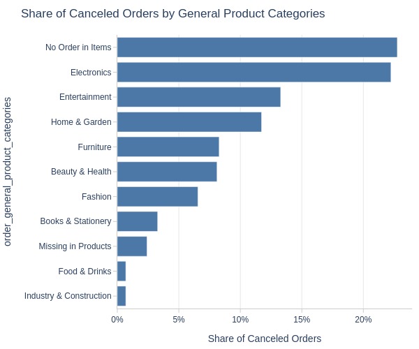
Key Observations:

• Top generalized canceled categories:

  1. Electronics

  2. Furniture

  3. Home & Garden

By Top Customer States

pb.bar_groupby(y='customer_state', text_auto=False)

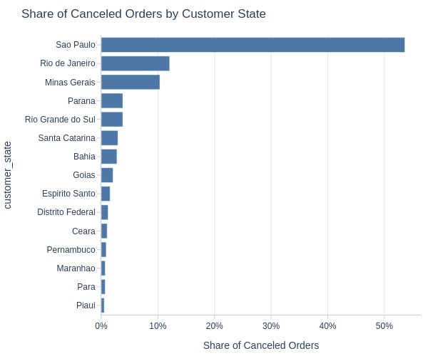
Key Observations:

• Canceled orders by state:

  • São Paulo: 42%

  • Rio: 13%

  • Minas: 12%

  • Others: ≤6%

Sum of Orders

By month

pb.configure(
    df = df_canceled
    , time_column = 'order_purchase_dt'
    , time_column_label = 'Date'
    , metric = 'total_payment'
    , metric_label = 'Canceled Orders Amount, R$'
    , title_base = 'Canceled Orders Amount'
    , agg_func = 'sum'
    , freq = 'ME'
)
pb.line_resample()

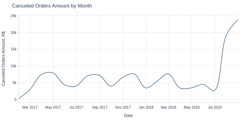
Key Observations:

• Canceled order revenue typically 4K-8K R$/month

• Anomalous spikes in Jul/Aug 2018

Average Order Value

By month

pb.configure(
    df = df_canceled
    , time_column = 'order_purchase_dt'
    , time_column_label = 'Date'
    , metric = 'total_payment'
    , metric_label = 'AOV (Canceled), R$'
    , title_base = 'AOV (Canceled)'
    , agg_func = 'mean'
    , freq = 'ME'
)
pb.line_resample()

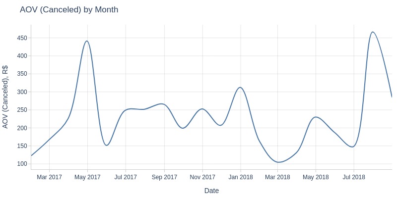
Key Observations:

• Canceled order value spikes in Apr 2017 and Jul 2018