Sales Analysis

Number of Sales

pb.configure(
    df = df_sales
    , time_column = 'order_purchase_dt'
    , time_column_label = 'Date' 
    , metric = 'order_id'
    , metric_label = 'Share of Sales'
    , metric_label_for_distribution = 'Number of Sales'
    , agg_func = 'nunique'
    , norm_by='all'
    , axis_sort_order='descending'
    , text_auto='.1%'
    , update_fig={'xaxis': {'tickformat': '.0%'}}
)

print(f'Total number of sales: {df_sales.order_id.nunique()}')

Total number of sales: 96346

Let’s see at statistics and distribution of the metric.

pb.metric_info(freq='D')

Summary Statistics for "nunique_order_id_per_day" (Type: Integer)

Summary			Percentiles			Detailed Stats			Value Counts
Total	602 (100%)		Max	1.15k		Mean	160.04		140	10 (2%)
Missing	---		99%	362.98		Trimmed Mean (10%)	155.10		149	7 (1%)
Distinct	255 (42%)		95%	293		Mode	140		72	7 (1%)
Non-Duplicate	90 (15%)		75%	214.75		Range	1143		103	7 (1%)
Duplicates	347 (58%)		50%	148.50		IQR	114.50		66	6 (<1%)
Dup. Values	165 (27%)		25%	100.25		Std	88.83		138	6 (<1%)
Zeros	---		5%	45		MAD	82.28		252	6 (<1%)
Negative	---		1%	10.01		Kurt	24.43		188	6 (<1%)
Memory Usage	<1 Mb		Min	4		Skew	2.57		145	6 (<1%)

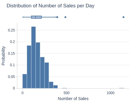
Key Observations:

• 75% of days had ≤215 orders

• 5% had ≤45 orders

• 5% had ≥293 orders

• Several days exceeded 400 orders

Let’s look by different dimensions.

By Season

Since 2018 has incomplete monthly data, it’s better to also analyze by year…

pb.bar_groupby(
    x='purchase_season'
    , color='purchase_year'
)

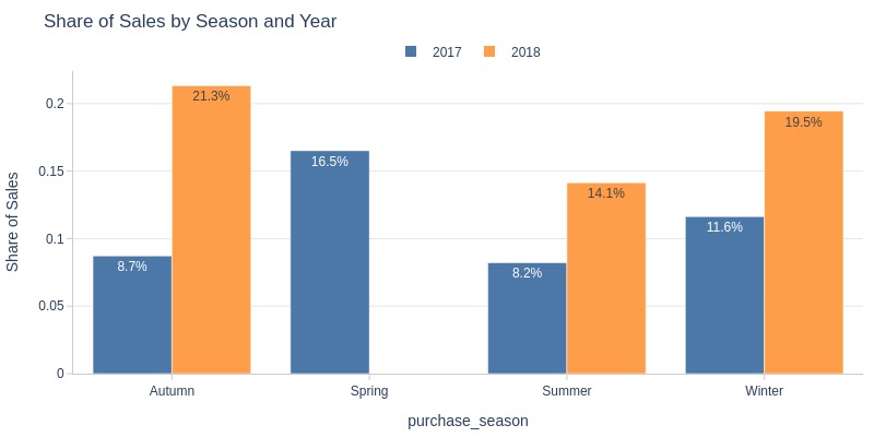
Key Observations:

• Lowest sales in summer (both years)

• Highest sales in autumn (2018)

By Time of Day

pb.bar_groupby(y='purchase_time_of_day')

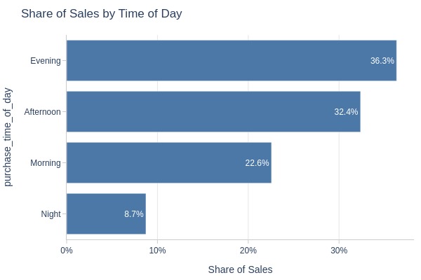
Key Observations:

• Sales by time of day:

  • Evening: 36% (peak)

  • Night: 9% (lowest)

  • Morning: 23%

  • Afternoon: 32%

By Day of Week

pb.bar_groupby(y='purchase_weekday')

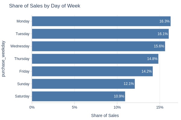
Key Observations:

• Saturday: 11% (lowest)

• Monday: 16% (highest)

By Weekday vs Weekend

pb.bar_groupby(y='purchase_day_type')

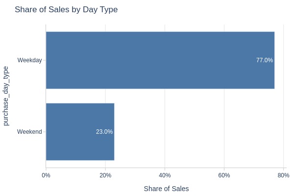
Key Observations:

• 77% of orders were placed on weekdays

By Day of the Week and Hour of the Day

fig = pb.heatmap(
    x='purchase_hour'
    , y='purchase_weekday'
    , labels={'color': 'Number of Sales'}
    , title='Number of Sales by Day of the Week and Hour of the Day'
).update_layout(xaxis_dtick=1, xaxis_tickformat=None)
pb.to_slide(fig)
fig.show()

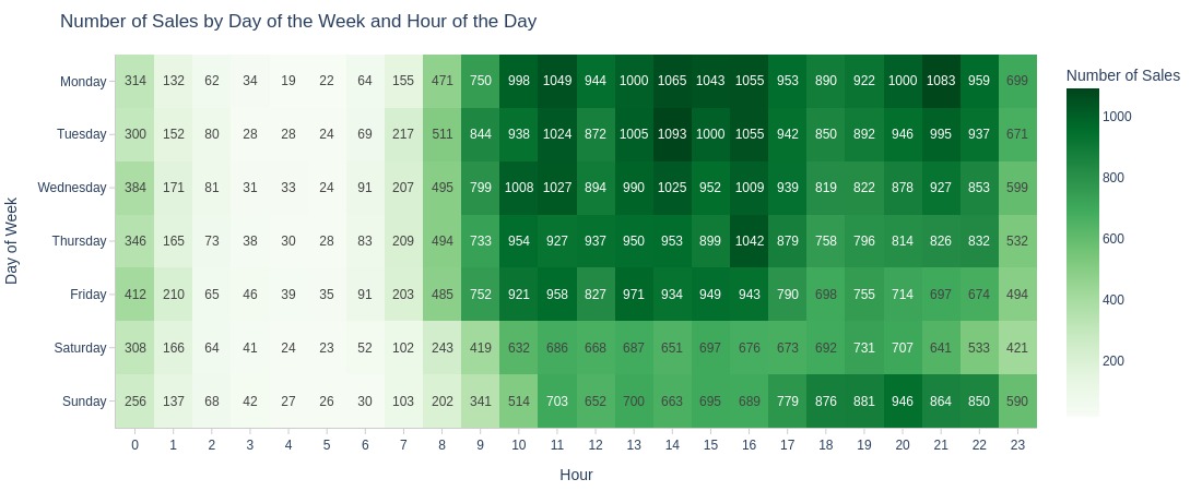
Key Observations:

• 1AM-8AM had lowest sales across all weekdays

By Review Score

pb.bar_groupby(y='order_avg_reviews_score')

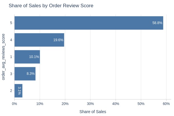
Key Observations:

• Review score distribution:

  • 5 stars: 59%

  • 2 stars: 3% (lowest)

  • More 1-star than 2/3-star orders

By Whether the Order is Delayed or Not

pb.bar_groupby(y='is_delayed')

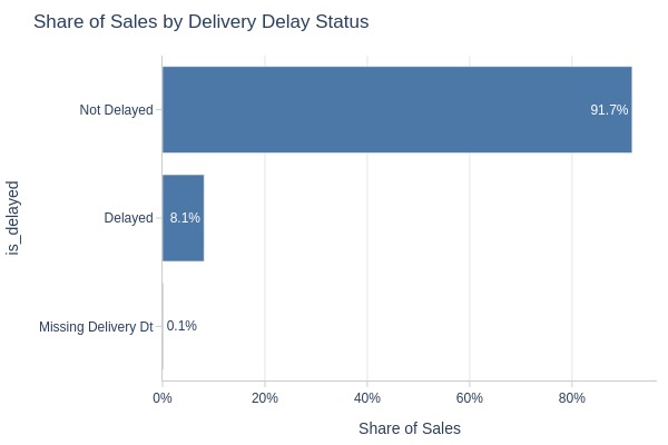
Key Observations:

• 92% of orders had no delivery delay

By Payment Category

pb.bar_groupby(y='order_total_payment_cat')

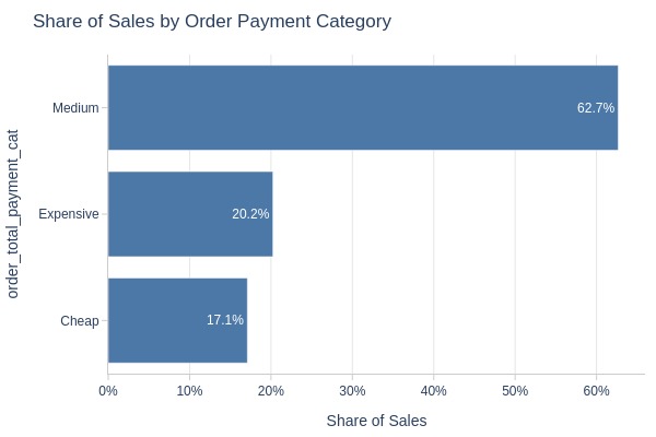
Key Observations:

• 63% of orders were medium-priced

By Order Weight Category

pb.bar_groupby(y='order_total_weight_cat')

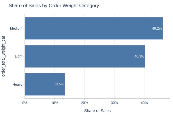
Key Observations:

• Order weight distribution:

  • Medium: 46%

  • Light: 40%

By Delivery Time Category

pb.bar_groupby(y='delivery_time_days_cat')

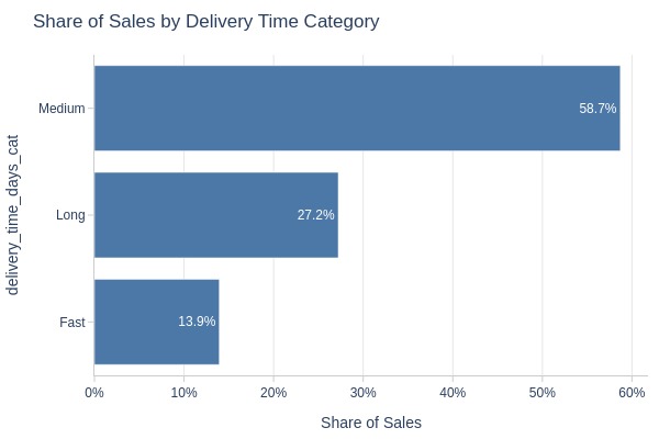
Key Observations:

• 59% of orders had medium delivery time

By Presence of Installment Payments

pb.bar_groupby(y='order_has_installment')

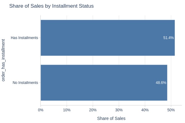
Key Observations:

• 51% of orders used installments

By Payment Type

pb.bar_groupby(y='order_payment_types')

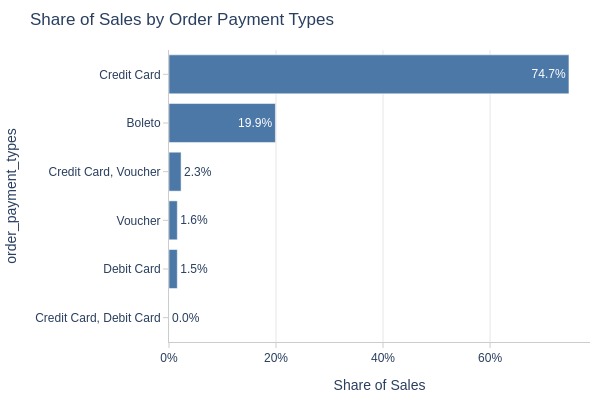
Key Observations:

• Payment methods:

  • Credit card: 75%

  • Boleto: 20%

By Product Category

pb.bar_groupby(
    y='order_product_categories'
    , text_auto=False
)

Key Observations:

• Top 3 product categories:

  1. Bed Bath Table: 9%

  2. Health Beauty: 9%

  3. Sports Leisure: 8%

By Generalized Product Category

pb.bar_groupby(
    y='order_general_product_categories'
    , text_auto=False
)

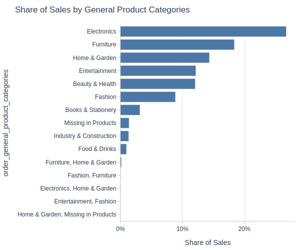
Key Observations:

• Top 3 generalized categories:

  1. Electronics: 27%

  2. Furniture: 18%

  3. Home & Garden: 14%

By Top Customer States

pb.bar_groupby(y='customer_state', text_auto=False)

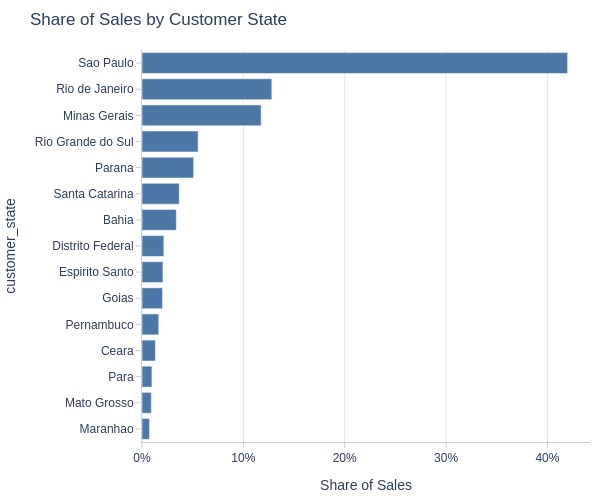
Key Observations:

• Sales by state:

  • São Paulo: 42%

  • Rio de Janeiro: 13%

  • Minas Gerais: 12%

  • Others: ≤6%

By Top Customer Cities

pb.bar_groupby(y='customer_city', text_auto=False)

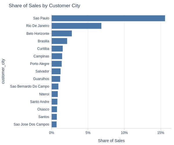
Key Observations:

• Sales by city:

  • São Paulo: 16%

  • Rio de Janeiro: 7%

  • Others: ≤3%

Sum of Sales

pb.configure(
    df = df_sales
    , time_column = 'order_purchase_dt'
    , metric = 'total_payment'
    , metric_label = 'Sum of Sales, R$'
    , agg_func = 'sum'
    , title_base = 'Sum and Number of Sales'
    , axis_sort_order='descending'
    , text_auto='.3s'
    , update_fig={'xaxis2': {'title_text': 'Number of Sales'}}
)

print(f'Total Sales Amount: {df_sales.total_payment.sum():,.2f}, R$')

Total Sales Amount: 15,399,404.87, R$

Let’s see at statistics and distribution of the metric.

pb.metric_info(freq='D')

Summary Statistics for "sum_total_payment_per_day" (Type: Float)

Summary			Percentiles			Detailed Stats			Value Counts
Total	602 (100%)		Max	175.25k		Mean	25.58k		707.27	1 (<1%)
Missing	---		99%	57.35k		Trimmed Mean (10%)	24.72k		27687.48	1 (<1%)
Distinct	602 (100%)		95%	48.90k		Mode	Multiple		39162.30	1 (<1%)
Non-Duplicate	602 (100%)		75%	33.76k		Range	174.74k		35845.39	1 (<1%)
Duplicates	---		50%	23.46k		IQR	18.59k		31531.31	1 (<1%)
Dup. Values	---		25%	15.17k		Std	14.28k		34643.87	1 (<1%)
Zeros	---		5%	6.73k		MAD	13.47k		24342.08	1 (<1%)
Negative	---		1%	1.57k		Kurt	19.15		25377.01	1 (<1%)
Memory Usage	<1 Mb		Min	507.85		Skew	2.22		27569.29	1 (<1%)

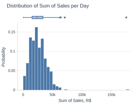
Key Observations:

• 75% of days had sales ≤33K R$

• 5% of days had ≤6.7K R$

• 5% of days had ≥49K R$

• Several days exceeded 70K R$

Let’s look by different dimensions.

By Season

Since 2018 has incomplete monthly data, it’s better to also analyze by year…

pb.bar_groupby(
    x='purchase_season'
    , color='purchase_year'
    , title='Sum of Sales by Season and Year'
)

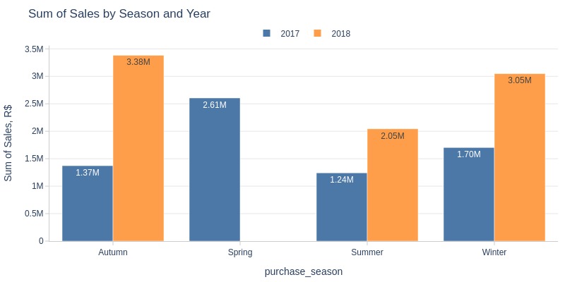
Key Observations:

• Lowest sales revenue in summer (both years)

• Highest revenue in autumn (2018)

By Time of Day

pb.bar_groupby(y='purchase_time_of_day', show_count=True, to_slide=True)

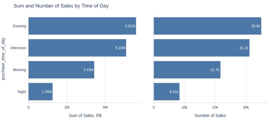
Key Observations:

• Highest sales volume and revenue in evenings

• Lowest at night

By Day of Week

pb.bar_groupby(y='purchase_weekday', show_count=True, to_slide=True)

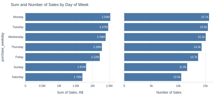
Key Observations:

• Monday has highest sales volume/revenue

• Saturday has lowest

By Weekday vs Weekend

pb.bar_groupby(y='purchase_day_type', show_count=True, to_slide=True)

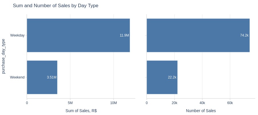
Key Observations:

• Weekday sales/revenue significantly higher than weekends

By Day of the Week and Hour of the Day

fig = pb.heatmap(
    x='purchase_hour'
    , y='purchase_weekday'
    , text_auto='.3s'
    , labels={'color': 'Amount, R$'}
    , title='Sales Amount by Day of the Week and Hour of the Day'
).update_layout(xaxis_dtick=1)
pb.to_slide(fig)
fig.show()

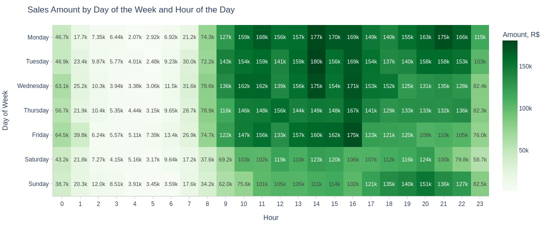
Key Observations:

• 1AM-8AM has lowest revenue across all weekdays

By Whether the Order is Delayed or Not

pb.bar_groupby(y='is_delayed', show_count=True)

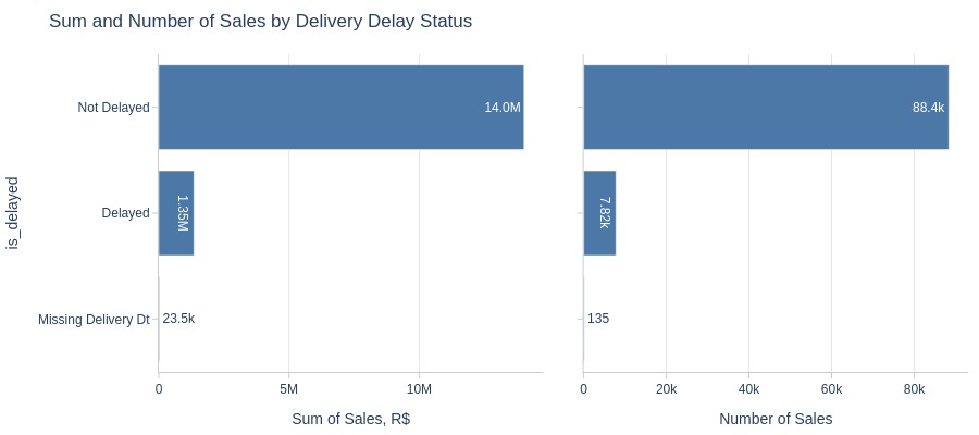
Key Observations:

• Non-delayed orders have significantly higher sales/revenue

By Order Weight Category

pb.bar_groupby(y='order_total_weight_cat', show_count=True, to_slide=True)

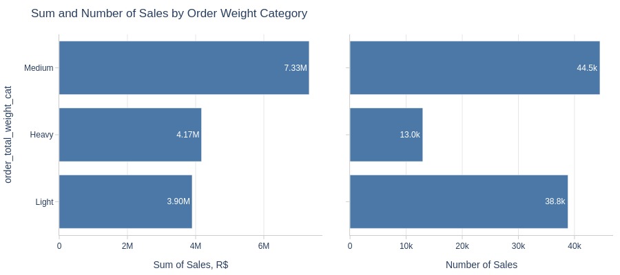
Key Observations:

• Medium-weight orders generate more revenue than heavy/light

• Light orders have higher quantity share but lower revenue share

• Heavy orders are more expensive

By Presence of Installment Payments

pb.bar_groupby(y='order_has_installment', show_count=True, to_slide=True)

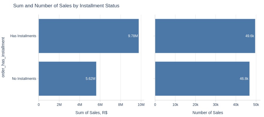
Key Observations:

• Installment orders generate significantly more revenue despite similar order counts

• Installment enables more expensive purchases

By Top Customer States

pb.bar_groupby(y='customer_state', show_count=True, to_slide=True)

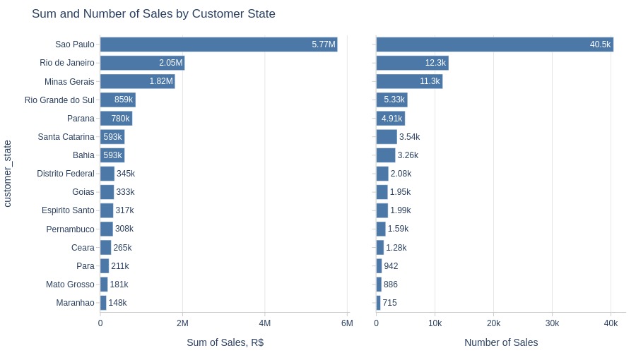
Key Observations:

• São Paulo state dominates sales volume/revenue

• Rio de Janeiro and Minas Gerais rank 2nd/3rd

By Top Customer Cities

pb.bar_groupby(y='customer_city', show_count=True, to_slide=True)

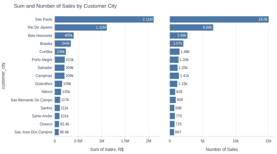
Key Observations:

• São Paulo city leads in sales volume/revenue

• Rio de Janeiro ranks second

By Review Score

pb.bar_groupby(y='order_avg_reviews_score', show_count=True, to_slide=True)

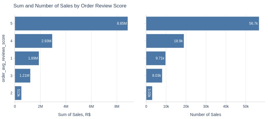
Key Observations:

• 5-star reviews have highest sales/revenue

• 2-star reviews have lowest

• 1-star reviews exceed 2/3-star in volume/revenue

By Payment Type

Since a single order can have multiple payments, we will measure transaction volume based on payment count.

pb.bar_groupby(
    y='order_payment_types'
    , show_count=True
    , to_slide=True
)

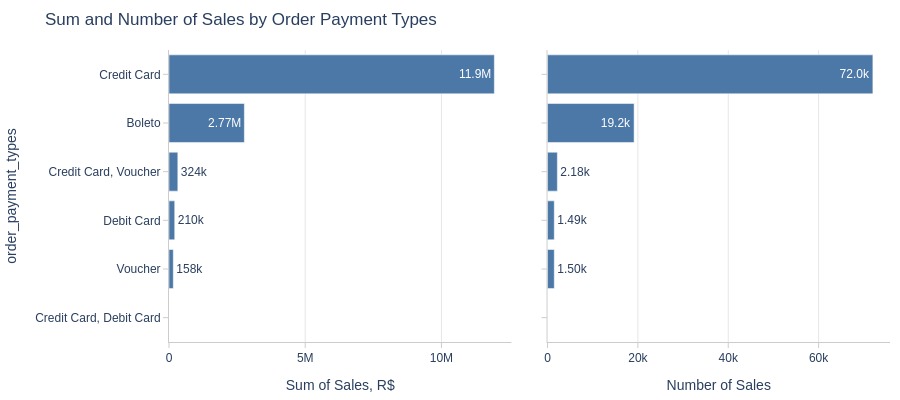
Key Observations:

• Credit card leads payment methods (volume/revenue)

• Boleto ranks second

By Product Category

For the category product split, we cannot take the payment amount. We will calculate the sum based on the product price and freight value.

The count will be determined by the number of items.

pb.bar_groupby(
    y='order_general_product_categories'
    , show_count=True
    , to_slide=True
)

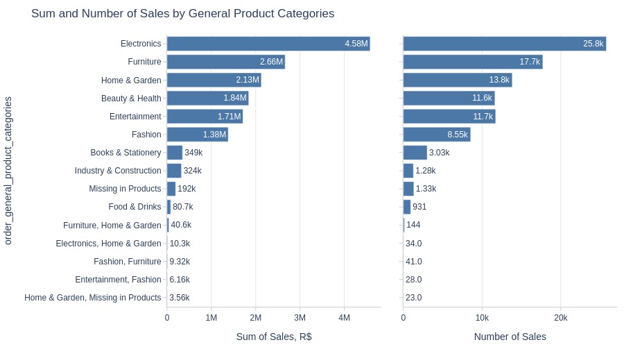
Key Observations:

• Electronics leads categories (volume/revenue)

• Furniture ranks second

• Furniture has smaller price gap in quantity vs revenue

Average Order Value

pb.configure(
    df = df_sales
    , metric = 'total_payment'
    , metric_label = 'Average Order Value, R$'
    , metric_label_for_distribution = 'Order Value, R$'
    , agg_func = 'mean'
    , title_base = 'Average Order Value and Number of Sales'
    , axis_sort_order='descending'
    , text_auto='.3s'
    , update_fig={'xaxis2': {'title_text': 'Number of Sales'}}    
)

Top Orders

pb.metric_top()

	total_payment
order_id
03caa2c082116e1d31e67e9ae3700499	13,664.08
736e1922ae60d0d6a89247b851902527	7,274.88
0812eb902a67711a1cb742b3cdaa65ae	6,929.31
fefacc66af859508bf1a7934eab1e97f	6,922.21
f5136e38d1a14a4dbd87dff67da82701	6,726.66
2cc9089445046817a7539d90805e6e5a	6,081.54
a96610ab360d42a2e5335a3998b4718a	4,950.34
199af31afc78c699f0dbf71fb178d4d4	4,764.34
8dbc85d1447242f3b127dda390d56e19	4,681.78
426a9742b533fc6fed17d1fd6d143d7e	4,513.32

Let’s see at statistics and distribution of the metric.

pb.metric_info(
    labels=dict(total_payment='Order Value, R$')
    , title='Distribution of Order Value'
    , upper_quantile=0.95
    , hist_mode='dual_hist_trim'
)

Summary Statistics for "total_payment" (Type: Float)

Summary			Percentiles			Detailed Stats			Value Counts
Total	96.35k (100%)		Max	13.66k		Mean	159.83		77.57	250 (<1%)
Missing	---		99%	1.05k		Trimmed Mean (10%)	119.85		35	164 (<1%)
Distinct	27.40k (28%)		95%	445.84		Mode	77.57		73.34	161 (<1%)
Non-Duplicate	12.82k (13%)		75%	176.26		Range	13.65k		116.94	131 (<1%)
Duplicates	68.94k (72%)		50%	105.28		IQR	114.36		56.78	118 (<1%)
Dup. Values	14.59k (15%)		25%	61.89		Std	218.93		107.78	118 (<1%)
Zeros	---		5%	32.38		MAD	76.37		65	112 (<1%)
Negative	---		1%	22.38		Kurt	249.10		86.15	106 (<1%)
Memory Usage	1		Min	9.59		Skew	9.37		99.90	105 (<1%)

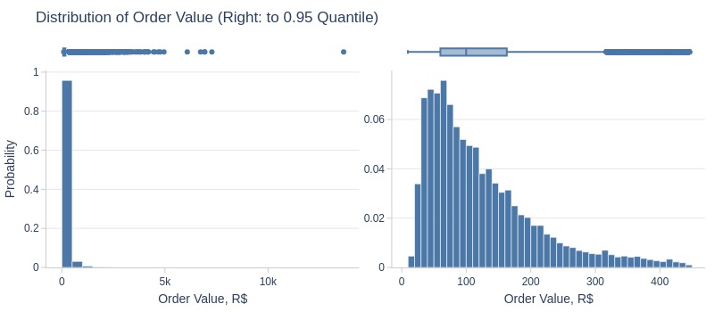
Key Observations:

• 75% of orders ≤177 R$

• 5% ≤33 R$

• 5% ≥445 R$

• Many outliers >1000 R$

Let’s look by different dimensions.

By Season

Since 2018 has incomplete monthly data, it’s better to also analyze by year…

pb.bar_groupby(
    x='purchase_season'
    , color='purchase_year'
    , title='Average Order Value by Season and Year'
)

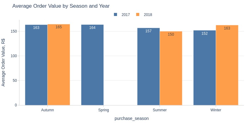
Key Observations:

• Summer 2017 had higher order values

• Other seasons slightly higher in 2018

By Day of the Week and Hour of the Day

fig = pb.heatmap(
    x='purchase_hour'
    , y='purchase_weekday'
    , text_auto='.1f'
    , labels={'color': 'AOV, R$'}
    , title='Average Order Value by Day of the Week and Hour of the Day'
).update_layout(xaxis_dtick=1)
pb.to_slide(fig)
fig.show()

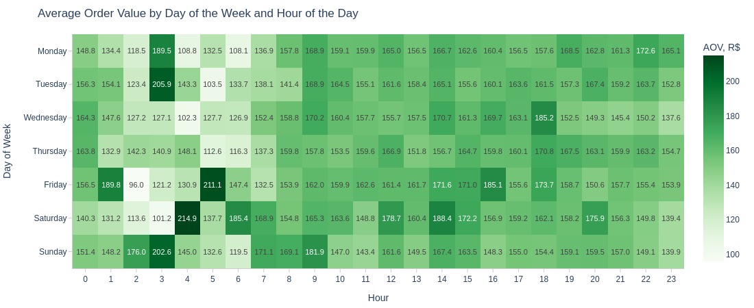
Key Observations:

• Nighttime doesn’t always have lowest average order value

• Some weekday nights show value peaks

By Whether the Order is Delayed or Not

pb.histogram(
    color='is_delayed'
    , upper_quantile=0.95
    , mode='dual_box_trim'
    , show_box=True
    , show_hist=True
    , show_kde=False
    , nbins=30
).show()
pb.bar_groupby(
    y='is_delayed'
    , show_count=True
).show()

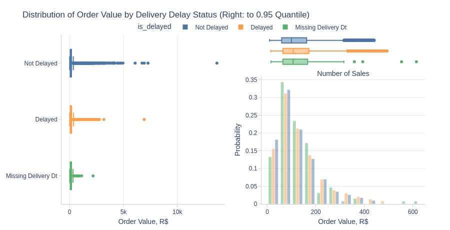
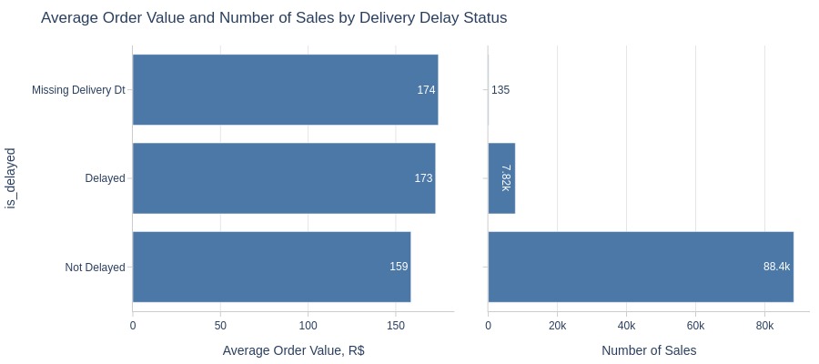
Key Observations:

• Non-delayed orders have lower average values

By Order Weight Category

pb.histogram(
    color='order_total_weight_cat'
    , upper_quantile=0.95
    , mode='dual_box_trim'
    , show_box=True
    , show_hist=True
    , show_kde=False
    , nbins=30
).show()
pb.bar_groupby(
    y='order_total_weight_cat'
    , show_count=True
).show()

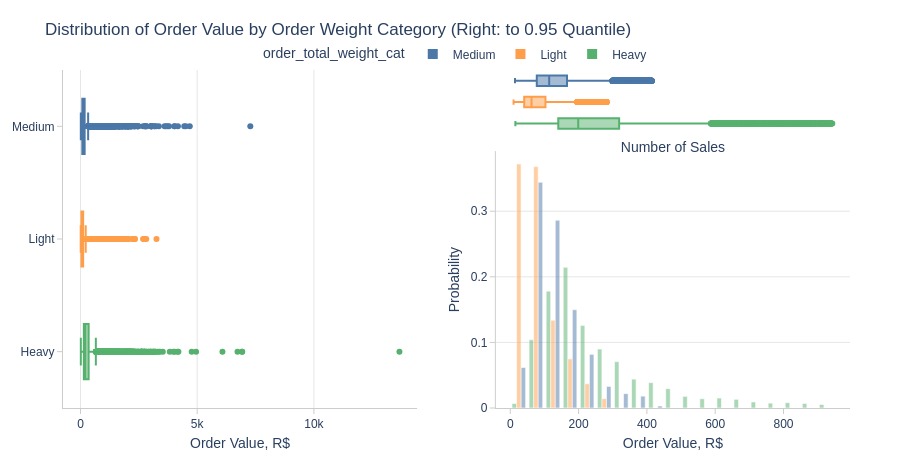
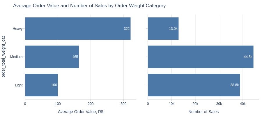
Key Observations:

• Heavier orders have higher average values

By Presence of Installment Payments

pb.histogram(
    color='order_has_installment'
    , upper_quantile=0.95
    , mode='dual_box_trim'
    , show_box=True
    , show_hist=True
    , show_kde=False
    , nbins=30
).show()
pb.bar_groupby(
    y='order_has_installment'
    , show_count=True
    , to_slide=True
).show()

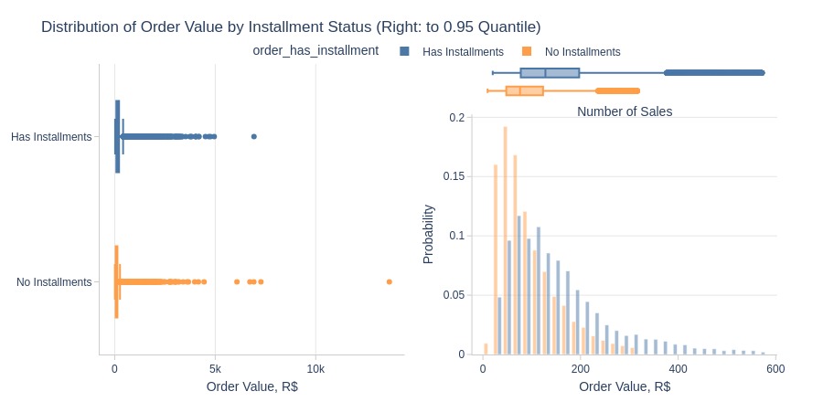
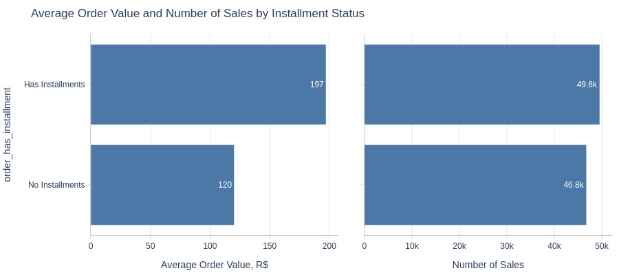
Key Observations:

• Installment orders have much higher average values

By Top Customer States

pb.box(
    y='customer_state'
    , upper_quantile=0.95
    , show_dual=True
).show()
pb.bar_groupby(
    y='customer_state'
    , show_count=True
    , to_slide=True
).show()

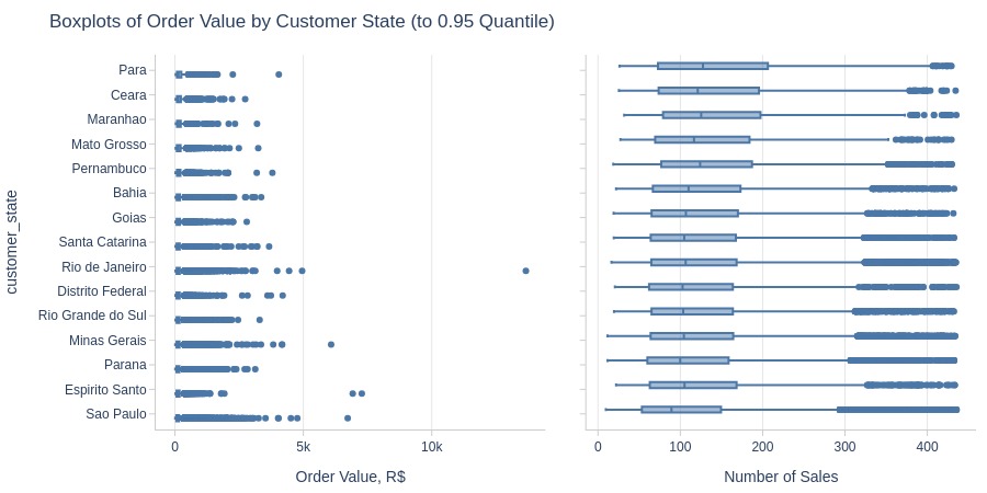
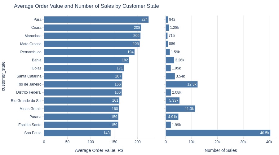
Key Observations:

• São Paulo has most orders but lowest average value among top states

• Para has highest average order value

By Top Customer Cities

pb.box(
    y='customer_city'
    , upper_quantile=0.95
    , show_dual=True
).show()
pb.bar_groupby(
    y='customer_city'
    , show_count=True
    , to_slide=True
).show()

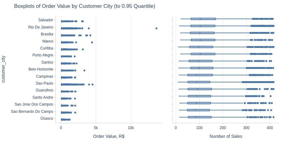
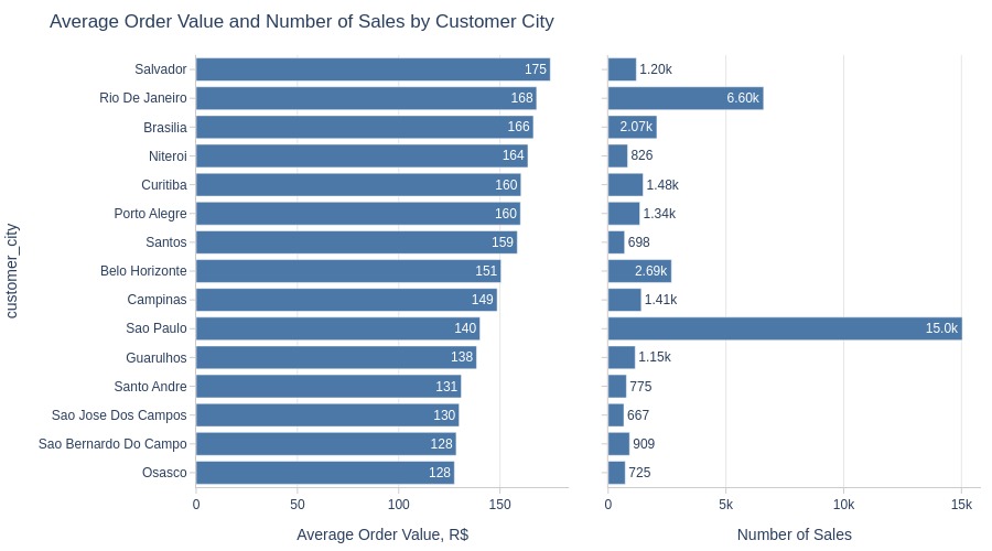
Key Observations:

• Rio de Janeiro combines high volume with high average value

• Salvador has highest average order value among top cities

By Review Score

pb.histogram(
    color='order_avg_reviews_score'
    , upper_quantile=0.95
    , mode='dual_box_trim'
    , show_box=True
    , show_hist=False
    , show_kde=True
    , nbins=30
).show()
pb.bar_groupby(
    y='order_avg_reviews_score'
    , show_count=True
    , to_slide=True
).show()

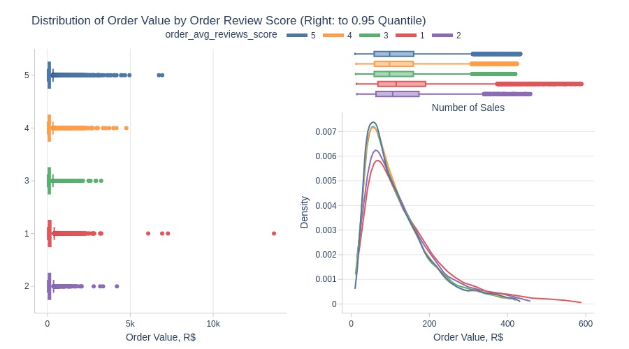
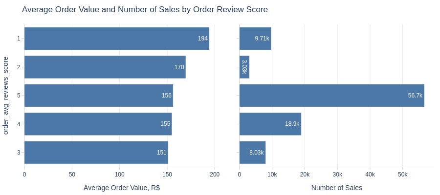
Key Observations:

• 1-star reviews have highest order values

• 2-star reviews rank second

• Expensive orders receive more low ratings

Reviews Score

pb.configure(
    df = df_sales
    , metric = 'order_avg_reviews_score'
    , metric_label = 'Average Order Reviews Score'
    , metric_label_for_distribution = 'Order Reviews Score'
    , agg_func = 'mean'
    , title_base = 'Average Order Reviews Score and Number of Sales'
    , axis_sort_order='descending'
    , text_auto='.3s'
    , update_fig={'xaxis2': {'title_text': 'Number of Sales'}}        
)

Let’s see at statistics and distribution of the metric.

pb.metric_info(
    labels=dict(order_avg_reviews_score='Order Reviews Score')
    , title='Distribution of Order Reviews Score'
    , xaxis_type='category'
)

Summary Statistics for "order_avg_reviews_score" (Type: Integer)

Summary			Percentiles			Detailed Stats			Value Counts
Total	96.35k (100%)		Max	5		Mean	4.14		5	56.65k (59%)
Missing	---		99%	5		Trimmed Mean (10%)	4.42		4	18.93k (20%)
Distinct	5 (<1%)		95%	5		Mode	5		1	9.71k (10%)
Non-Duplicate	0 (<1%)		75%	5		Range	4		3	8.03k (8%)
Duplicates	96.34k (99%)		50%	5		IQR	1		2	3.03k (3%)
Dup. Values	5 (<1%)		25%	4		Std	1.30
Zeros	---		5%	1		MAD	0
Negative	---		1%	1		Kurt	0.84
Memory Usage	1		Min	1		Skew	-1.45

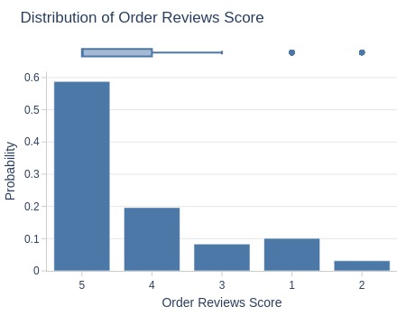
Key Observations:

• 59% of orders have 5-star reviews

Let’s look by different dimensions.

By Season

pb.bar_groupby(
    x='purchase_season'
    , color='purchase_year'
    , title='Average Order Reviews Score by Season and Year'
)

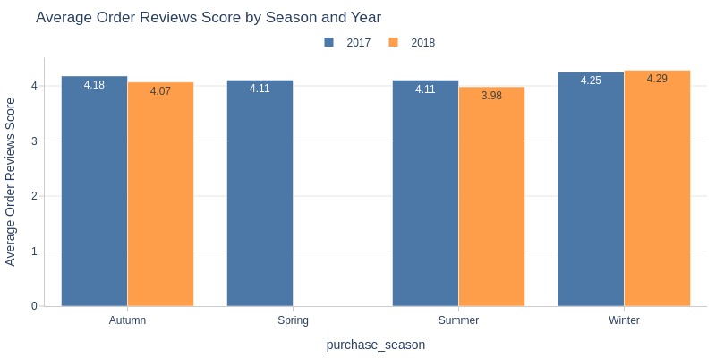
Key Observations:

• Winter 2018 had slightly higher ratings

• Other seasons slightly higher in 2017

By Day of the Week and Hour of the Day

pb.heatmap(
    x='purchase_hour'
    , y='purchase_weekday'
    , text_auto='.1f'
    , title='Average Order Reviews Score by Day of the Week and Hour of the Day'
    , labels=dict(color = 'Score')
).update_layout(xaxis_dtick=1)

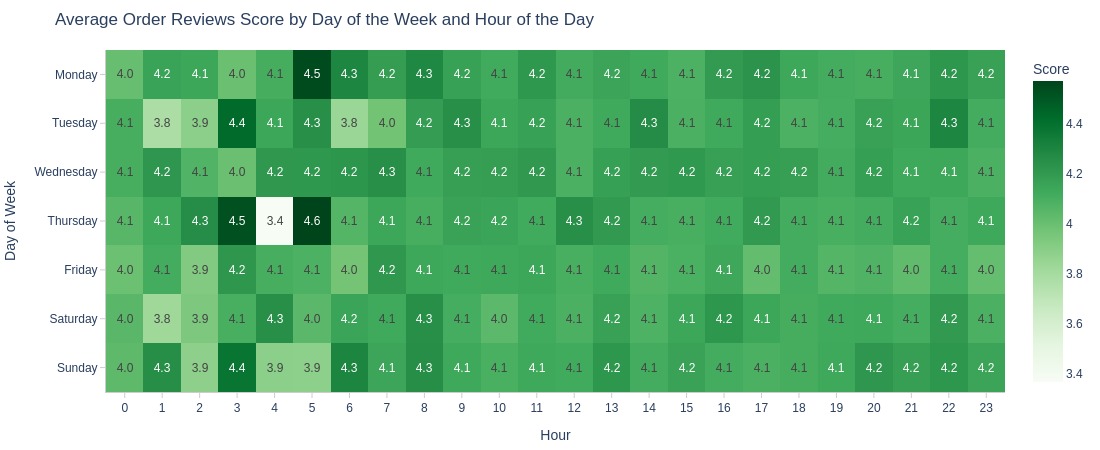
Key Observations:

• Nighttime shows rating extremes (especially Thursdays)

By Delivery Delay Status

pb.cat_compare(
    cat2='is_delayed'
    , visible_graphs=[2]
)
pb.bar_groupby(
    y='is_delayed'
    , show_count=True
    , to_slide=True
).show()

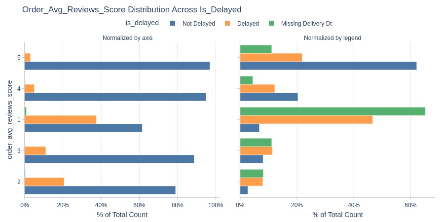
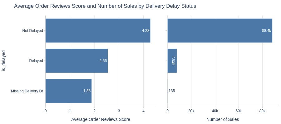
Key Observations:

• Non-delayed orders have significantly higher ratings

• Higher 5-star share for on-time deliveries

• “Unknown” delivery status orders mostly get 1-star

By Delivery Time Category

pb.cat_compare(
    cat2='delivery_time_days_cat'
    , visible_graphs=[2]
)
pb.bar_groupby(
    y='delivery_time_days_cat'
    , show_count=True
).show()

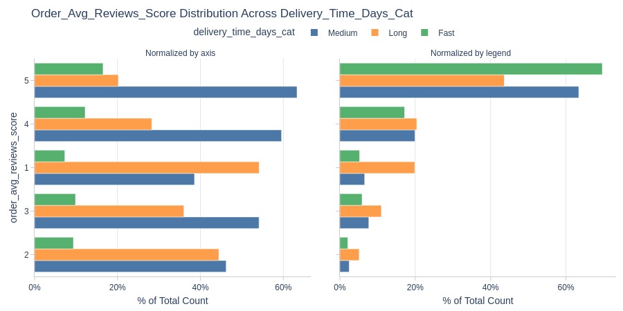
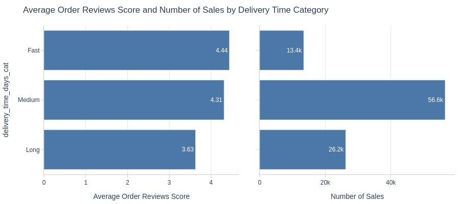
Key Observations:

• Faster deliveries get better ratings

By Customer State

pb.cat_compare(
    cat2='customer_state'
    , visible_graphs=[2]
    , trim_top_n_cat2=7
)
fig = pb.bar_groupby(
    y='customer_state'
    , show_count=True
).update_layout(xaxis_domain=[0, 0.4], xaxis2_domain=[0.6, 1])
pb.to_slide(fig)
fig.show()

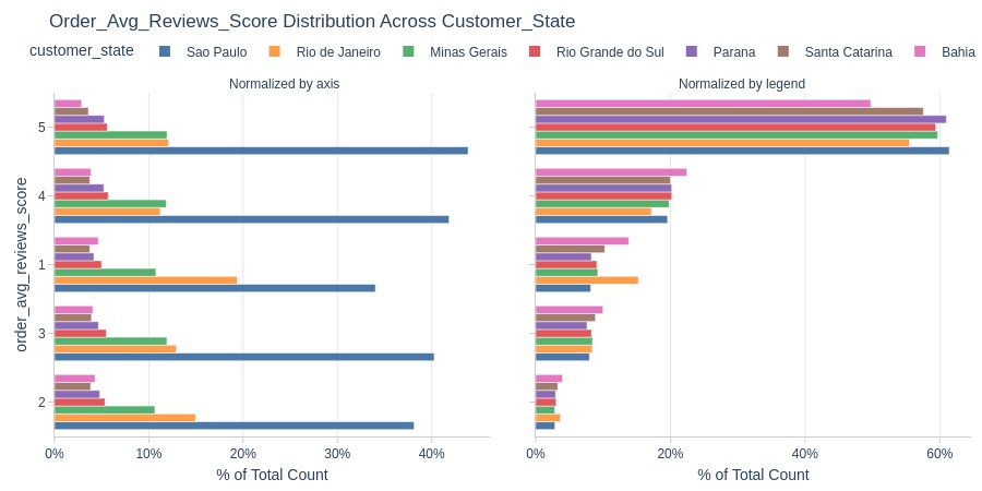
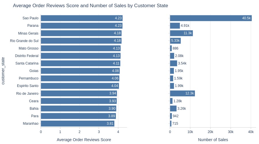
Key Observations:

• Maranhão has lowest average rating among top states

• Rio de Janeiro and Bahia have highest 1-star share

By Customer City

pb.cat_compare(
    cat2='customer_city'
    , visible_graphs=[2]
    , trim_top_n_cat2=7
)
pb.bar_groupby(
    y='customer_city'
    , show_count=True
).update_layout(xaxis_domain=[0, 0.4], xaxis2_domain=[0.6, 1]).show()

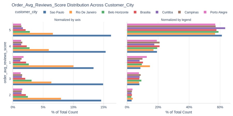
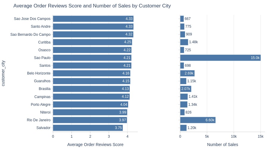
Key Observations:

• Rio de Janeiro and Porto Alegre have notable 1-star concentrations

Order Weight

pb.configure(
    df = df_sales
    , metric = 'total_weight_kg'
    , metric_label = 'Average Weight of Order, kg'
    , metric_label_for_distribution = 'Weight of Order, kg'
    , title_base = 'Average Weight of Order and Number of Sales'
    , agg_func = 'mean'
    , axis_sort_order='descending'
    , text_auto='.3s'
    , update_fig={'xaxis2': {'title_text': 'Number of Sales'}}        
)

Top Orders

pb.metric_top()

	total_weight_kg
order_id
9aec4e1ae90b23c7bf2d2b3bfafbd943	184.40
2455cbeb73fd04b170ca2504662f95ce	154.20
8f6f263a5e96515d5534199b74cb7748	144.30
be382a9e1ed25128148b97d6bfdb21af	129.34
cf4659487be50c0c317cff3564c4a840	112.20
53cbc02ffe278ca84b6f4920d9d3ecd5	108.50
60b570df9018c6b6441017314a2dd081	98.40
f60ce04ff8060152c83c7c97e246d6a8	97.00
1446ae966d68c3abad1ca3a3ce58033e	96.80
35990049382e07dba1a9ef3550cad655	93.90

Let’s see at statistics and distribution of the metric.

pb.metric_info(
    labels=dict(total_weight_kg='Weight of Order, kg')
    , title='Distribution of Weight of Order'
    , upper_quantile=0.99
    , hist_mode='dual_hist_trim'
)

Summary Statistics for "total_weight_kg" (Type: Float)

Summary			Percentiles			Detailed Stats			Value Counts
Total	96.35k (100%)		Max	184.40		Mean	2.39		0.20	5.36k (6%)
Missing	---		99%	22.35		Trimmed Mean (10%)	1.30		0.15	4.16k (4%)
Distinct	1.48k (2%)		95%	10.50		Mode	0.20		0.30	3.69k (4%)
Non-Duplicate	384 (<1%)		75%	2.05		Range	184.40		0.25	3.69k (4%)
Duplicates	94.87k (98%)		50%	0.75		IQR	1.75		0.40	3.30k (3%)
Dup. Values	1.09k (1%)		25%	0.30		Std	4.77		0.10	2.87k (3%)
Zeros	5 (<1%)		5%	0.15		MAD	0.82		0.35	2.75k (3%)
Negative	---		1%	0.10		Kurt	96.51		0.50	2.36k (2%)
Memory Usage	1		Min	0		Skew	6.58		0.60	2.27k (2%)

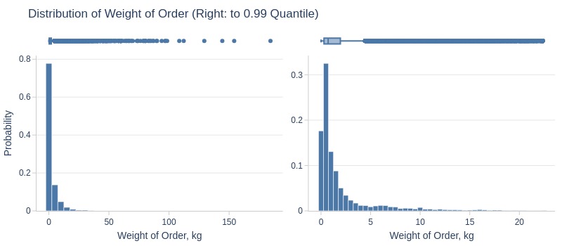
Key Observations:

• 75% of orders ≤2kg

• 5% ≤150g

• 5% ≥10kg

Let’s look by different dimensions.

By Season

Since 2018 has incomplete monthly data, it’s better to also analyze by year…

pb.bar_groupby(
    x='purchase_season'
    , color='purchase_year'
    , title='Average Weight of Order by Season and Year'
)

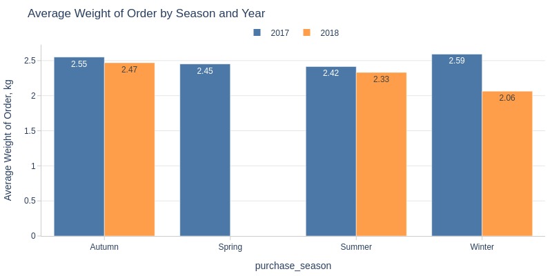
Key Observations:

• 2017 had heavier orders across all seasons

By Time of Day

pb.histogram(
    color='purchase_time_of_day'
    , upper_quantile=0.95
    , mode='dual_box_trim'
    , show_box=True
    , show_hist=False
    , show_kde=True
).show()
pb.bar_groupby(
    y='purchase_time_of_day'
    , show_count=True
).show()

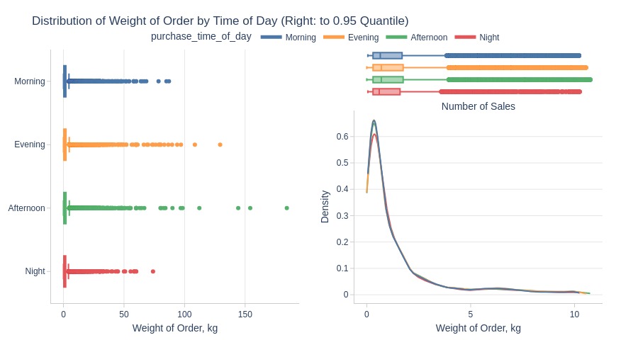
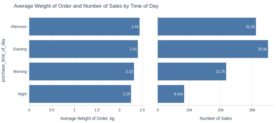
Key Observations:

• Afternoons have heaviest orders

• Nights have lightest

By Whether the Order is Delayed or Not

pb.histogram(
    color='is_delayed'
    , upper_quantile=0.95
    , mode='dual_box_trim'
    , show_box=True
    , show_hist=False
    , show_kde=True
).show()
pb.bar_groupby(
    y='is_delayed'
    , show_count=True
    , to_slide=True
).show()

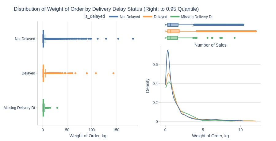
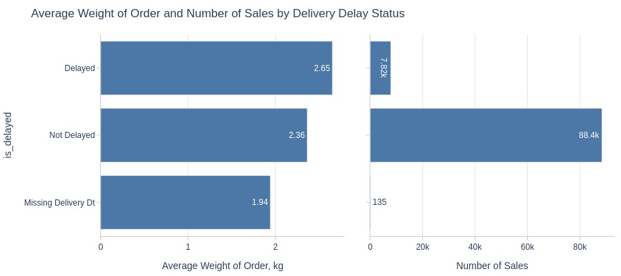
Key Observations:

• Delayed orders are heavier

By Presence of Installment Payments

pb.histogram(
    color='order_has_installment'
    , upper_quantile=0.95
    , mode='dual_box_trim'
    , show_box=True
    , show_hist=False
    , show_kde=True
).show()
pb.bar_groupby(
    y='order_has_installment'
    , show_count=True
    , to_slide=True
)

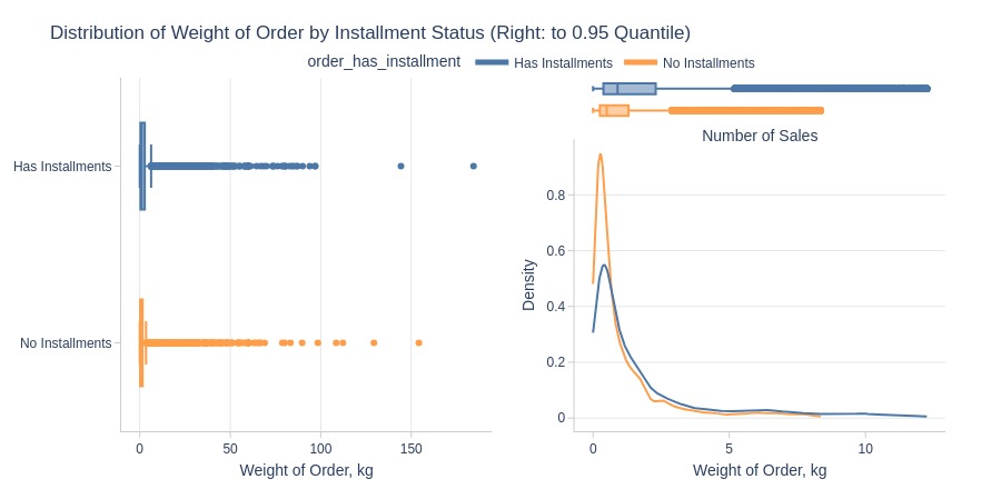
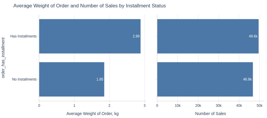
Key Observations:

• Installment orders are heavier

By Top Customer States

pb.box(
    y='customer_state'
    , upper_quantile=0.95
    , show_dual=True
).show()
pb.bar_groupby(
    y='customer_state'
    , show_count=True
    , to_slide=True
).show()

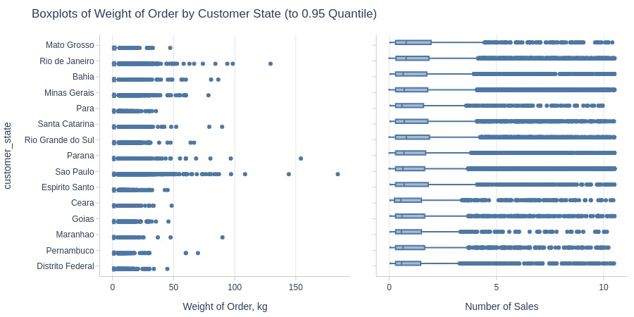
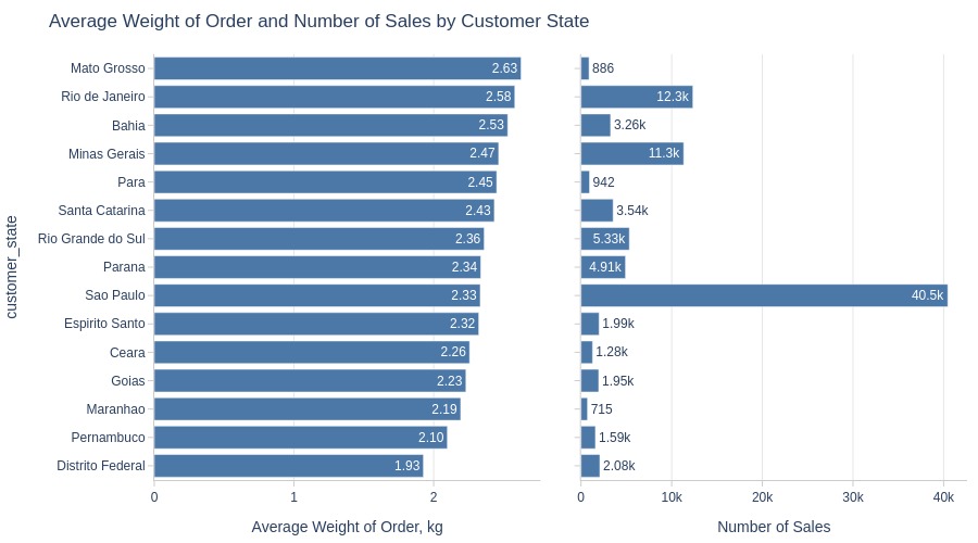
Key Observations:

• Mato Grosso has heaviest average orders among top states

By Top Customer Cities

pb.box(
    y='customer_city'
    , upper_quantile=0.95
    , show_dual=True
).show()
pb.bar_groupby(
    y='customer_city'
    , show_count=True
    , to_slide=True
)

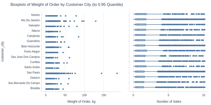
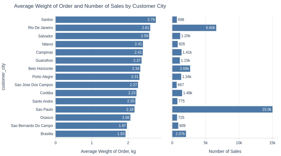
Key Observations:

• Santos and Rio de Janeiro have heaviest average orders

By Review Score

pb.bar_groupby(y='order_avg_reviews_score', show_count=True, to_slide=True)

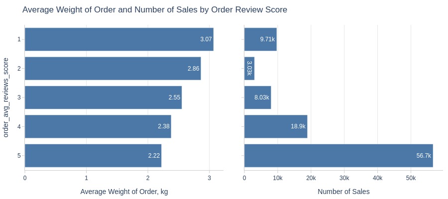
Key Observations:

• 1-star reviews have significantly heavier orders

• 2-star reviews rank second

• Heavy orders receive lower ratings

Number of Products per Order

pb.configure(
    df = df_sales
    , metric = 'products_cnt'
    , metric_label = 'Average Number of Products in Order'
    , metric_label_for_distribution = 'Number of Products in Order'
    , title_base = 'Number of Products in Order and Number of Sales'
    , agg_func = 'mean'
    , axis_sort_order='descending'
    , text_auto='.3s'
    , update_fig={'xaxis2': {'title_text': 'Number of Sales'}}          
)

Top Orders

pb.metric_top()

	products_cnt
order_id
8272b63d03f5f79c56e9e4120aec44ef	21.00
1b15974a0141d54e36626dca3fdc731a	20.00
ab14fdcfbe524636d65ee38360e22ce8	20.00
428a2f660dc84138d969ccd69a0ab6d5	15.00
9ef13efd6949e4573a18964dd1bbe7f5	15.00
9bdc4d4c71aa1de4606060929dee888c	14.00
73c8ab38f07dc94389065f7eba4f297a	14.00
37ee401157a3a0b28c9c6d0ed8c3b24b	13.00
2c2a19b5703863c908512d135aa6accc	12.00
af822dacd6f5cff7376413c03a388bb7	12.00

Let’s see at statistics and distribution of the metric.

pb.metric_info(
    labels=dict(products_cnt='Number of Products in Order')
    , title='Distribution of Number of Products in Order'
)

Summary Statistics for "products_cnt" (Type: Integer)

Summary			Percentiles			Detailed Stats			Value Counts
Total	96.35k (100%)		Max	21		Mean	1.14		1	86.74k (90%)
Missing	---		99%	3		Trimmed Mean (10%)	1		2	7.38k (8%)
Distinct	17 (<1%)		95%	2		Mode	1		3	1.30k (1%)
Non-Duplicate	2 (<1%)		75%	1		Range	20		4	493 (<1%)
Duplicates	96.33k (99%)		50%	1		IQR	0		5	192 (<1%)
Dup. Values	15 (<1%)		25%	1		Std	0.54		6	189 (<1%)
Zeros	---		5%	1		MAD	0		7	22 (<1%)
Negative	---		1%	1		Kurt	116.86		8	8 (<1%)
Memory Usage	1		Min	1		Skew	7.57		10	8 (<1%)

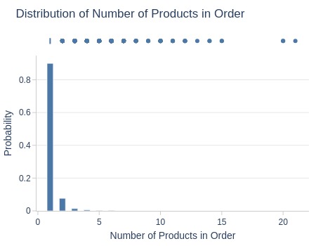
Key Observations:

• 90% of orders contain single product

• Two anomalies had 20-21 products

Let’s look by different dimensions.

By Whether the Order is Delayed or Not

pb.bar_groupby(
    y='is_delayed'
    , show_count=True
).show()

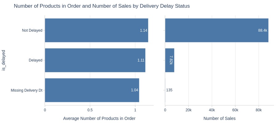
Key Observations:

• Non-delayed orders have slightly more products

By Review Score

pb.bar_groupby(y='order_avg_reviews_score', show_count=True, to_slide=True)

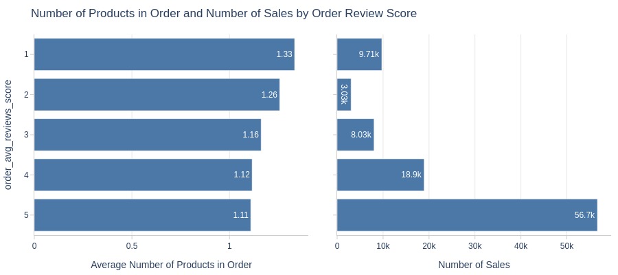
Key Observations:

• 1/2-star reviews have more products per order

Product Price per Order

pb.configure(
    df = df_sales
    , metric = 'avg_products_price'
    , metric_label = 'Average Product Price in Order, R$'
    , metric_label_for_distribution = 'Product Price in Order, R$'
    , agg_func = 'mean'
    , title_base = 'Average Product Price in Order and Number of Sales'
    , axis_sort_order='descending'
    , text_auto='.3s'
    , update_fig={'xaxis2': {'title_text': 'Number of Sales'}}         
)

Top Orders

pb.metric_top()

	avg_products_price
order_id
0812eb902a67711a1cb742b3cdaa65ae	6,735.00
fefacc66af859508bf1a7934eab1e97f	6,729.00
f5136e38d1a14a4dbd87dff67da82701	6,499.00
a96610ab360d42a2e5335a3998b4718a	4,799.00
199af31afc78c699f0dbf71fb178d4d4	4,690.00
8dbc85d1447242f3b127dda390d56e19	4,590.00
426a9742b533fc6fed17d1fd6d143d7e	4,399.87
68101694e5c5dc7330c91e1bbc36214f	4,099.99
b239ca7cd485940b31882363b52e6674	4,059.00
86c4eab1571921a6a6e248ed312f5a5a	3,999.90

Let’s see at statistics and distribution of the metric.

pb.metric_info(
    labels=dict(avg_products_price='Average Product Price in Order, R$')
    , title='Distribution of Average Product Price in Order'
    , upper_quantile=0.99
    , hist_mode='dual_hist_trim'
)

Summary Statistics for "avg_products_price" (Type: Float)

Summary			Percentiles			Detailed Stats			Value Counts
Total	96.35k (100%)		Max	6.74k		Mean	125.24		59.90	1.96k (2%)
Missing	---		99%	899.90		Trimmed Mean (10%)	90.41		69.90	1.70k (2%)
Distinct	7.01k (7%)		95%	362.86		Mode	59.90		49.90	1.58k (2%)
Non-Duplicate	3.51k (4%)		75%	139.90		Range	6.73k		89.90	1.30k (1%)
Duplicates	89.34k (93%)		50%	79		IQR	97.95		99.90	1.23k (1%)
Dup. Values	3.50k (4%)		25%	41.95		Std	189.82		39.90	1.07k (1%)
Zeros	---		5%	18.49		MAD	63.90		29.90	1.04k (1%)
Negative	---		1%	10.99		Kurt	119.27		79.90	1.04k (1%)
Memory Usage	1		Min	0.85		Skew	7.87		19.90	990 (1%)

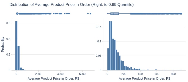
Key Observations:

• 75% of orders have average product price ≤140 R$

• 5% have ≥363 R$

Let’s look by different dimensions.

By Season

Since 2018 has incomplete monthly data, it’s better to also analyze by year…

pb.bar_groupby(
    x='purchase_season'
    , color='purchase_year'
    , title='Average Product Price in Order by Season and Year'
)

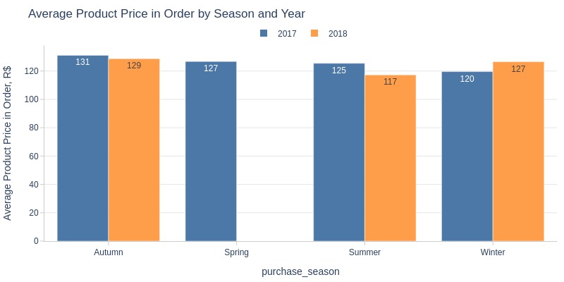
Key Observations:

• Summer/fall 2017 had higher product prices

• Winter 2018 was higher

By Time of Day

pb.histogram(
    color='purchase_time_of_day'
    , upper_quantile=0.95
    , mode='dual_box_trim'
    , show_box=True
    , show_hist=False
    , show_kde=True
).show()
pb.bar_groupby(
    y='purchase_time_of_day'
    , show_count=True
).show()

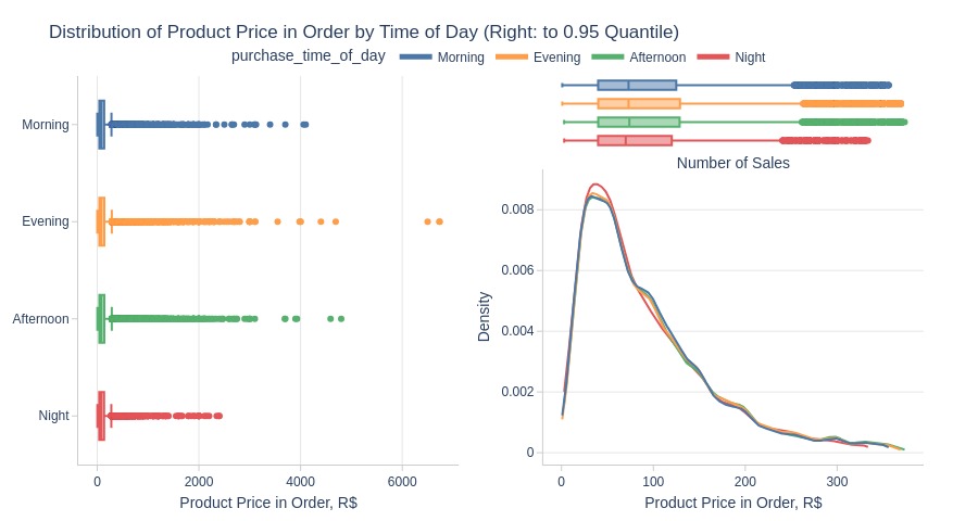
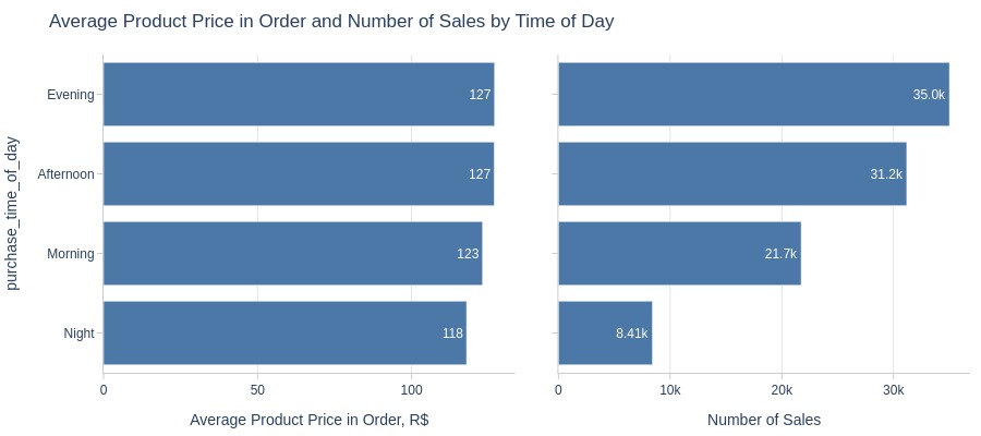
Key Observations:

• Nighttime has lower product prices

By Whether the Order is Delayed or Not

pb.histogram(
    color='is_delayed'
    , upper_quantile=0.95
    , mode='dual_box_trim'
    , show_box=True
    , show_hist=False
    , show_kde=True
).show()
pb.bar_groupby(
    y='is_delayed'
    , show_count=True
).show()

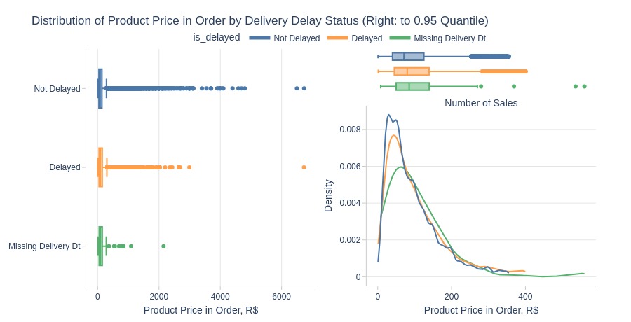
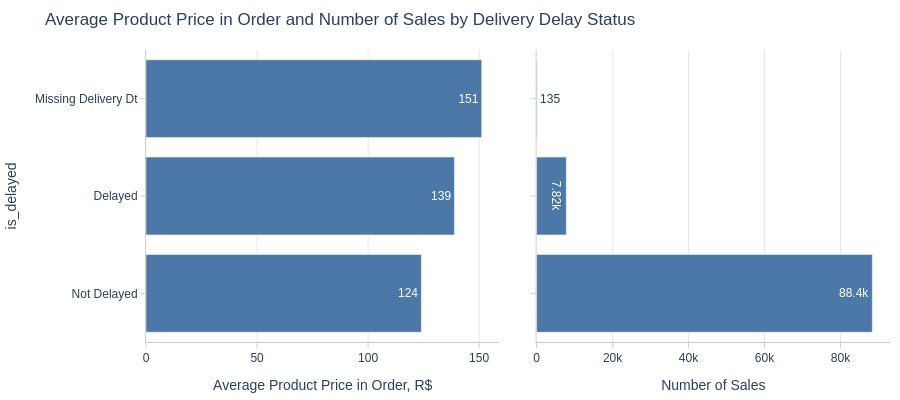
Key Observations:

• Delayed orders have higher product prices

By Presence of Installment Payments

pb.histogram(
    color='order_has_installment'
    , upper_quantile=0.95
    , mode='dual_box_trim'
    , show_box=True
    , show_hist=False
    , show_kde=True
).show()
pb.bar_groupby(
    y='order_has_installment'
    , show_count=True
    , to_slide=True
).show()

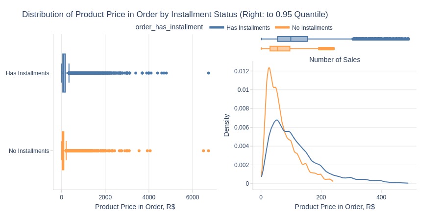
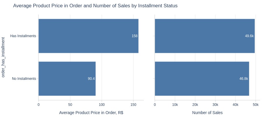
Key Observations:

• Installment orders have significantly higher product prices

By Top Customer States

pb.box(
    y='customer_state'
    , upper_quantile=0.95
    , show_dual=True
).show()
pb.bar_groupby(
    y='customer_state'
    , show_count=True
).show()

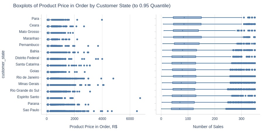
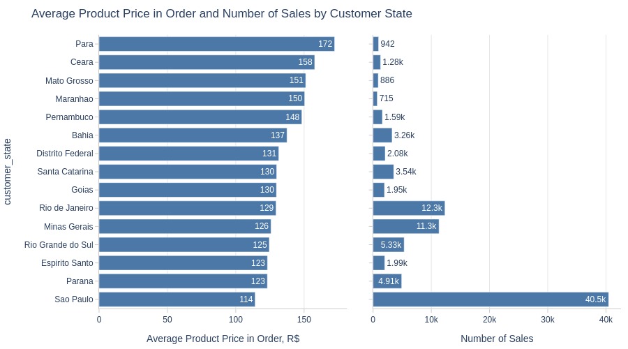
Key Observations:

• Para has highest average product price among top states

• São Paulo has lowest

By Top Customer Cities

pb.box(
    y='customer_city'
    , upper_quantile=0.95
    , show_dual=True
).show()
pb.bar_groupby(
    y='customer_city'
    , show_count=True
).show()

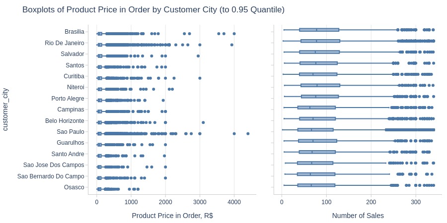
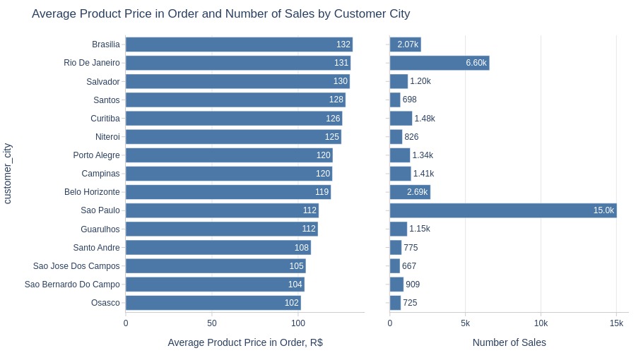
Key Observations:

• Brasília, Rio de Janeiro and Salvador have highest product prices among top cities.

Number of Sellers per Order

pb.configure(
    df = df_sales
    , metric = 'sellers_cnt'
    , metric_label = 'Average Number of Sellers in Order'
    , agg_func = 'mean'
    , axis_sort_order='descending'
)

Top Orders

pb.metric_top()

	sellers_cnt
order_id
1c11d0f4353b31ac3417fbfa5f0f2a8a	5.00
cf5c8d9f52807cb2d2f0a0ff54c478da	5.00
91be51c856a90d7efe86cf9d082d6ae3	4.00
8c2b13adf3f377c8f2b06b04321b0925	4.00
1d23106803c48c391366ff224513fb7f	4.00
338ffe54b65a3b8124c81ebe6d1cc4b0	3.00
a8c403407745aac434946d5058faa6a6	3.00
ffb8f7de8940249a3221252818937ecb	3.00
30bdf3d824d824610a49887486debcaf	3.00
3040863957c9336e7389512584639bb5	3.00

Let’s see at statistics and distribution of the metric.

pb.metric_info(
    labels=dict(sellers_cnt='Number of Sellers in Order')
    , title='Distribution of Number of Sellers in Order'
    , xaxis_type='category'
)

Summary Statistics for "sellers_cnt" (Type: Integer)

Summary			Percentiles			Detailed Stats			Value Counts
Total	96.35k (100%)		Max	5		Mean	1.01		1	95.07k (99%)
Missing	---		99%	2		Trimmed Mean (10%)	1		2	1.21k (1%)
Distinct	5 (<1%)		95%	1		Mode	1		3	54 (<1%)
Non-Duplicate	0 (<1%)		75%	1		Range	4		4	3 (<1%)
Duplicates	96.34k (99%)		50%	1		IQR	0		5	2 (<1%)
Dup. Values	5 (<1%)		25%	1		Std	0.12
Zeros	---		5%	1		MAD	0
Negative	---		1%	1		Kurt	118.85
Memory Usage	1		Min	1		Skew	9.88

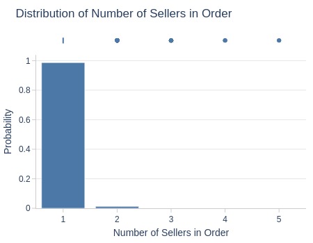
Key Observations:

• 99% of orders have single seller

Number of Categories per Order

pb.configure(
    df = df_sales
    , metric = 'product_categories_cnt'
    , metric_label = 'Average Number of Categories in Order'
    , agg_func = 'mean'
    , axis_sort_order='descending'
)

Top Orders

pb.metric_top()

	product_categories_cnt
order_id
8c2b13adf3f377c8f2b06b04321b0925	3.00
e8c92cfd87f5f0c6d2fc5bc1df5f02b4	3.00
1fcbc88015c88c1a14d4b8ec35ea8ed7	3.00
91be51c856a90d7efe86cf9d082d6ae3	3.00
4ca4a1922b582950b25cce6e7ef34315	3.00
2f8f31eb2f7b6572836d662a6625c8e4	3.00
ceb35b18f6b84c1c75f02859ce3160d9	3.00
cbb7694680a105281d391bf7002c0477	3.00
6616fa4c89b8bf2a7e17271cdc542fca	3.00
d4bec1a24c97bd17be18d77297a0f6a0	3.00

Let’s see at statistics and distribution of the metric.

pb.metric_info(
    labels=dict(product_categories_cnt='Number of Categories in Order')
    , title='Distribution of Number of Categories in Order'
    , xaxis_type='category'
)

Summary Statistics for "product_categories_cnt" (Type: Integer)

Summary			Percentiles			Detailed Stats			Value Counts
Total	96.35k (100%)		Max	3		Mean	1.01		1	95.57k (99%)
Missing	---		99%	1		Trimmed Mean (10%)	1		2	760 (<1%)
Distinct	3 (<1%)		95%	1		Mode	1		3	18 (<1%)
Non-Duplicate	0 (<1%)		75%	1		Range	2
Duplicates	96.34k (99%)		50%	1		IQR	0
Dup. Values	3 (<1%)		25%	1		Std	0.09
Zeros	---		5%	1		MAD	0
Negative	---		1%	1		Kurt	141.03
Memory Usage	1		Min	1		Skew	11.56

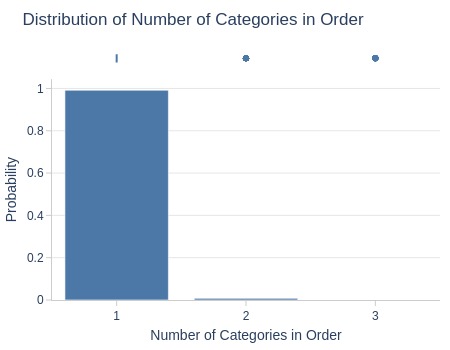
Key Observations:

• 99% of orders have single category