Geographical Analysis

Geo-analysis by ZIP Codes

Data Preparation

We will aggregate data by the first 3 digits of the customer’s ZIP code. Each point on the map will represent a unique truncated ZIP code.

Without truncation, we would get excessive detail and no noticeable differences.

We will prepare the data for visualization.

We have 6 orders that were made outside South America.

After truncating the prefixes, we may get additional coordinates outside South America.

We will remove them to avoid interfering with the map analysis.

tmp_df_res = df_sales.copy()
tmp_df_res['is_delayed'] = tmp_df_res['is_delayed'] == 'Delayed'
tmp_df_res['order_has_installment'] = tmp_df_res['order_has_installment'] == 'Has Installments'

tmp_df_res = (
    tmp_df_res.merge(df_customers_origin[['customer_id', 'customer_zip_code_prefix_3_digits']], on='customer_id')
    .groupby('customer_zip_code_prefix_3_digits', as_index=False)
    .agg(
        total_orders=('order_id', 'nunique')
        , orders_delayed_share = ('is_delayed', 'mean')
        , total_payment = ('total_payment', 'sum')
        , aov = ('total_payment', 'mean')
        , avg_installments = ('total_installments_cnt', 'mean')
        , first_orders_cnt = ('sale_is_customer_first_purchase', 'sum')
        , installment_orders_cnt = ('order_has_installment', 'sum')
        , total_reviews = ('reviews_cnt', 'sum')
        , avg_review_score = ('order_avg_reviews_score', 'mean')
        , avg_delivery_delay_days = ('delivery_delay_days', 'mean')
        , avg_delivery_time_days = ('delivery_time_days', 'mean')
        , avg_products_cnt = ('products_cnt', 'mean')
        , avg_freight_ratio = ('freight_ratio', 'mean')
        , avg_order_weight_kg = ('total_weight_kg', 'mean')
        , avg_order_volume_cm3 = ('total_volume_cm3', 'mean')
    ) 
)

tmp_df_res = (
    df_orders.assign(
        is_canceled = lambda x: x.order_status=='Canceled'
    )
    .merge(df_customers_origin, on='customer_unique_id')
    .groupby('customer_zip_code_prefix_3_digits', as_index=False)
    .agg(
        cancel_rate = ('is_canceled', 'mean')
    )
    .merge(tmp_df_res, on='customer_zip_code_prefix_3_digits', how='right')
    .merge(df_geolocations[lambda x:x.in_south_america], left_on = 'customer_zip_code_prefix_3_digits', right_on='geolocation_zip_code_prefix_3_digits')
)

tmp_df_res['repeat_purchase_rate'] = (tmp_df_res['total_orders'] - tmp_df_res['first_orders_cnt']) / tmp_df_res['total_orders']
tmp_df_res['installment_orders_rate'] = tmp_df_res['installment_orders_cnt'] / tmp_df_res['total_orders']

We will calculate the average MAU by the truncated ZIP code.

temp_mau = (
    df_sales.merge(df_customers_origin[['customer_id', 'customer_zip_code_prefix_3_digits']], on='customer_id')
    .groupby(['customer_zip_code_prefix_3_digits', pd.Grouper(key='order_purchase_dt', freq='ME')], observed=False)
    .agg(mau = ('customer_unique_id', 'nunique'))
    .groupby('customer_zip_code_prefix_3_digits', observed=False)
    .mean()
)
tmp_df_res = tmp_df_res.merge(temp_mau, on='customer_zip_code_prefix_3_digits', how='left')

del temp_mau

Data Visualization

We will create labels for displaying on the maps.

labels_for_map = dict(
    total_orders = 'Number of Sales'
    , total_payment = 'Sales Amount, R$'
    , aov = 'Average Order Value, R$'
    , mau = 'MAU'
    , avg_freight_ratio = 'Average Freight Ratio'
    , avg_delivery_time_days = 'Average Delivery Time, days'
    , avg_review_score = 'Average Review Score'
    , orders_delayed_share = 'Percentage of Delayed Orders'
    , avg_products_cnt = 'Average Number of Products in Order'
    , installment_orders_rate = 'Installment Payment Rate'
    , avg_installments = 'Average Number of Installments in Order'
    , avg_order_weight_kg = 'Average Order Weight, kg'
    , avg_order_volume_cm3 = 'Average Order Volume, cm3'
    , repeat_purchase_rate = 'Repeat Purchase Rate'
    , cancel_rate = 'Cancel Rate'
    , geolocation_lat = 'Latitude'
    , geolocation_lng = 'Longitude'
    , customer_zip_code_prefix_3_digits = 'Zip Code Prefix'
)

We will create a function for visualization.

def plot_map_zip(metric: str):
    """Create plotly map by 3-digit zip code prefix"""
    title = f"Distribution of {labels_for_map[metric].split(',')[0]} by 3-Digit Zip Code Prefix"
    colorbar_title = labels_for_map[metric].split(',')[1] if ',' in labels_for_map[metric] else None
    hover_data = {'geolocation_lat': False, 'geolocation_lng': False, 'customer_zip_code_prefix_3_digits': True}
    is_percentage = metric in [
        'avg_freight_ratio', 'orders_delayed_share', 
        'installment_orders_rate', 'repeat_purchase_rate', 
        'cancel_rate']
    if metric != 'total_orders':
        hover_data['total_orders'] = ':.2s'
    if not is_percentage:
        hover_data[metric] = ':.2s'
    else:
        hover_data[metric] = ':.1%'
    fig = px.scatter_map(
        tmp_df_res,
        lat='geolocation_lat',
        lon='geolocation_lng',
        color=metric,
        labels=labels_for_map,
        zoom=3,
        height=650,
        hover_data=hover_data,
        width=700,
        title=title,
        color_continuous_scale="matter",
        center={"lat": -14.235004, "lon": -55.92528}
    )
    if is_percentage:
        fig.update_coloraxes(
            colorbar_tickformat=".0%"
        )
    fig.update_layout(
        margin = dict(l=10, r=10, b=10, t=30)
        , title_y=0.99
        , coloraxis_colorbar_title_text = colorbar_title
    )
    pb.to_slide(fig)
    return fig

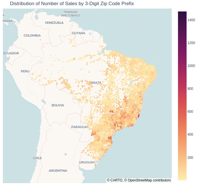
Where are the sales volume higher?

plot_map_zip('total_orders')

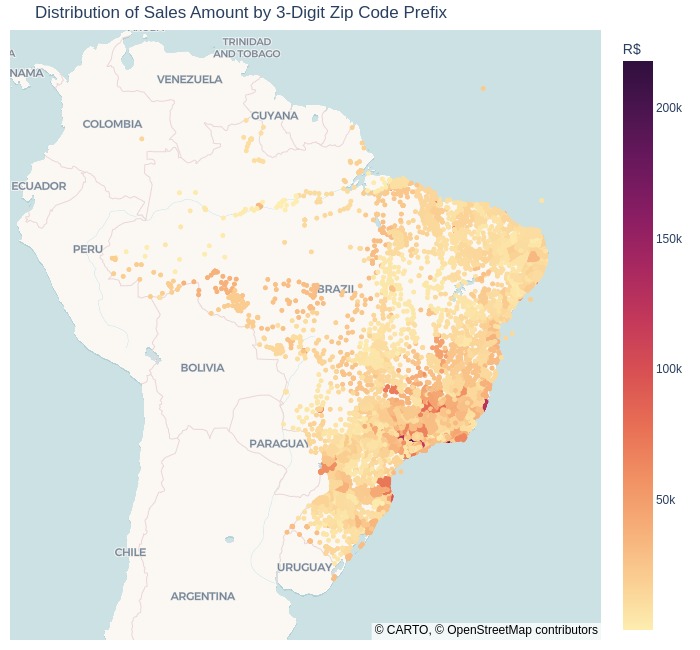
Where is the sales amount higher?

plot_map_zip('total_payment')

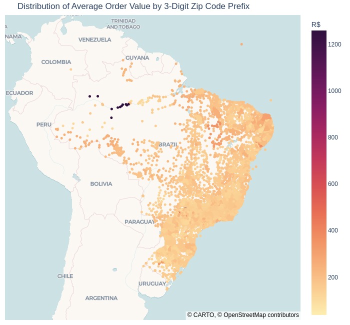
Where is the average order value higher?

plot_map_zip('aov')

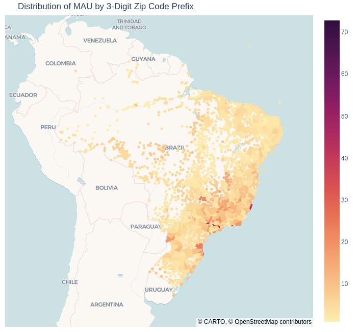
Where is average MAU higher?

plot_map_zip('mau')

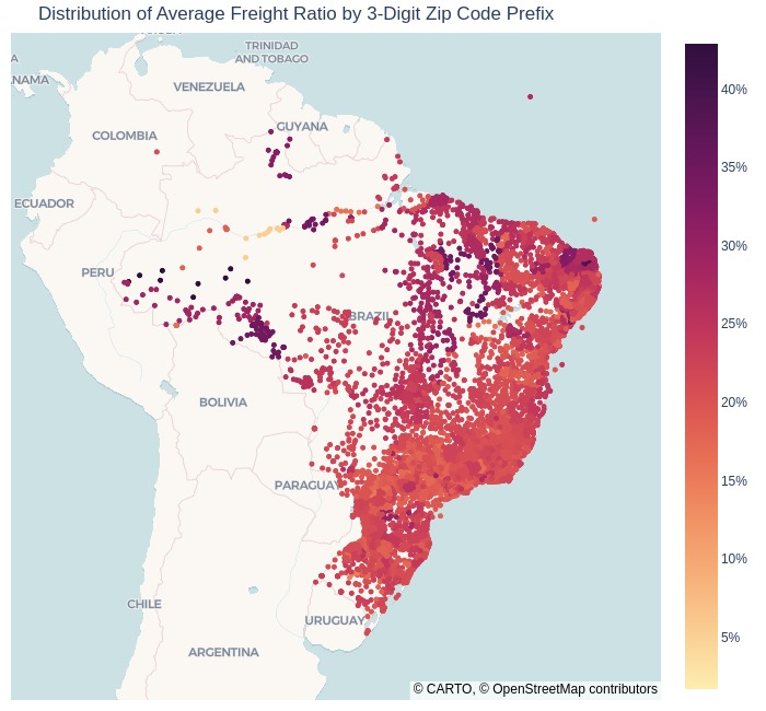
Where do customers pay more for delivery?

plot_map_zip('avg_freight_ratio')

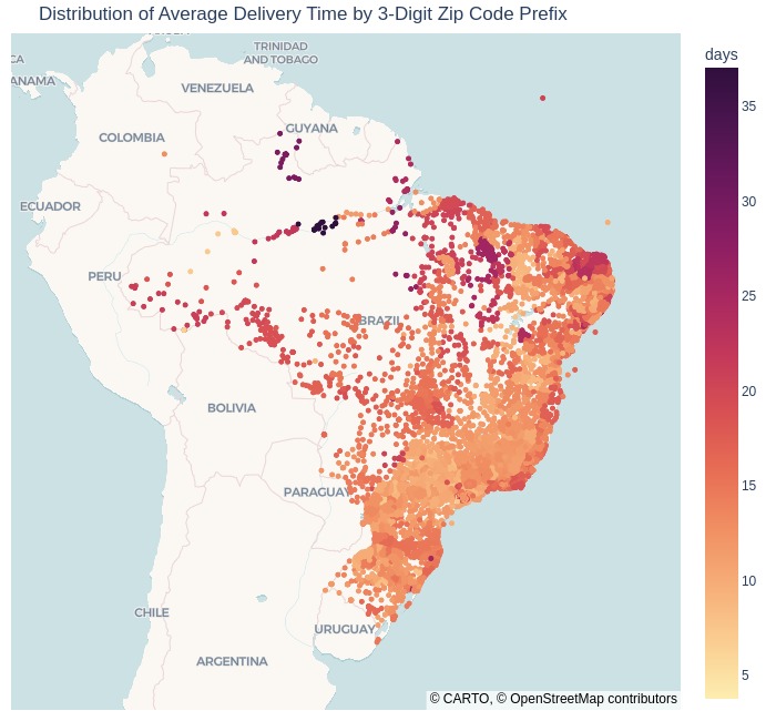
How is delivery time distributed across regions?

plot_map_zip('avg_delivery_time_days')

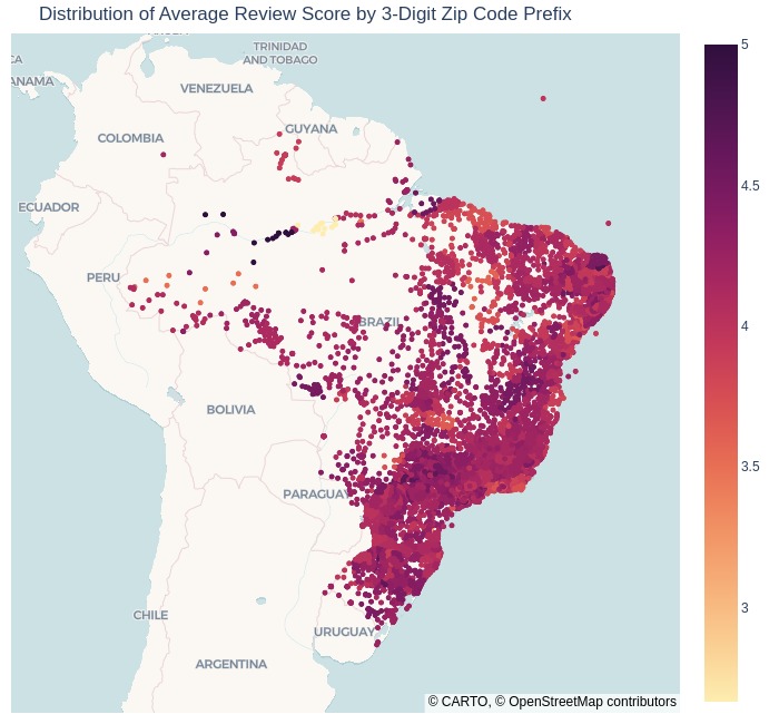
What is the average rating by regions?

plot_map_zip('avg_review_score')

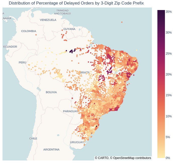
How are delayed orders distributed across regions?

plot_map_zip('orders_delayed_share')

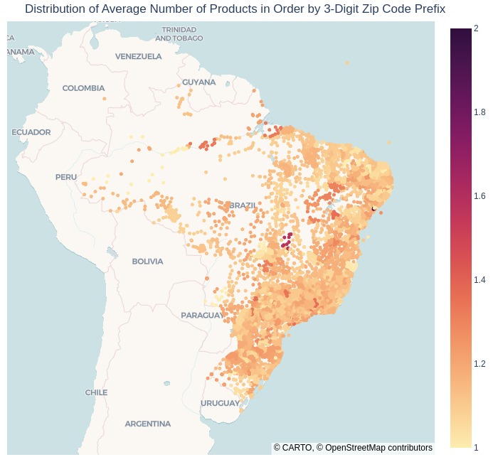
How is the number of items per order distributed across regions?

plot_map_zip('avg_products_cnt')

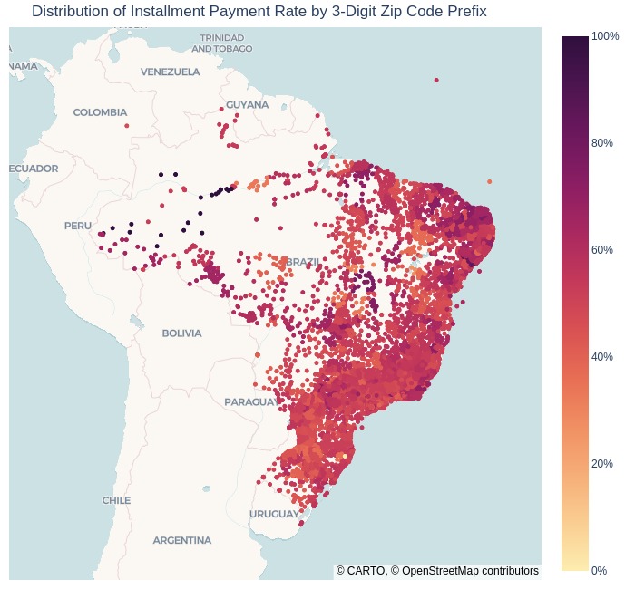
What is the higher proportion of installment payments in which regions?

plot_map_zip('installment_orders_rate')

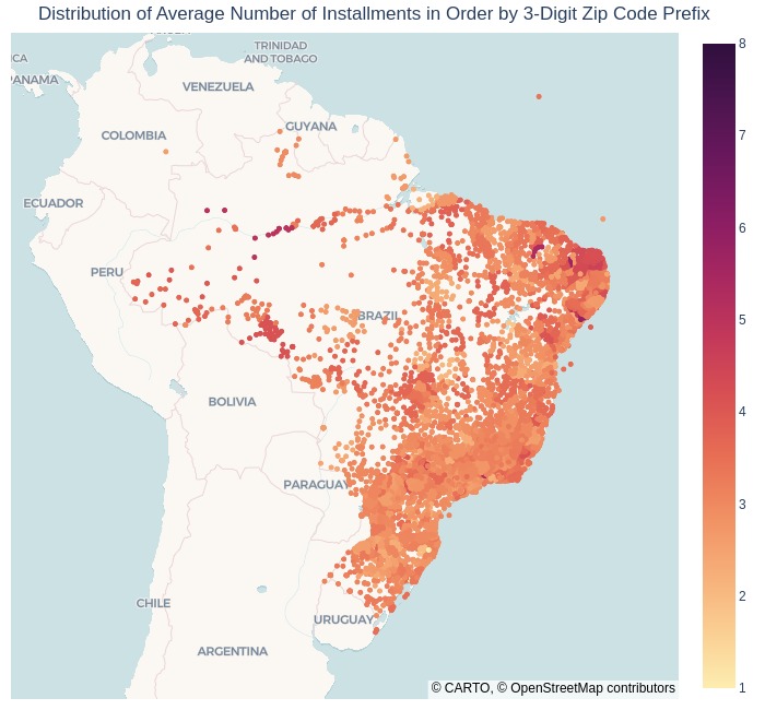
What regions have more installments per order?

plot_map_zip('avg_installments')

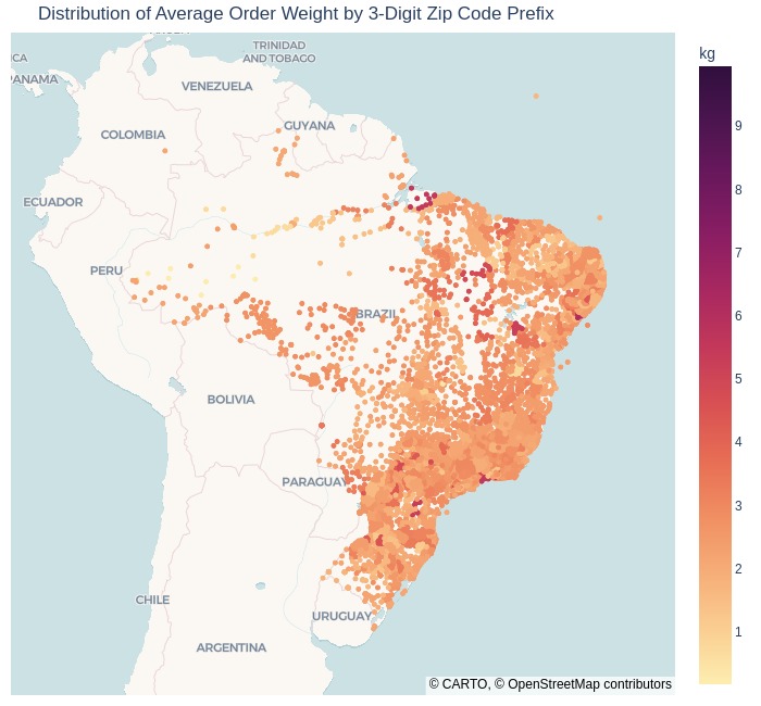
What regions have the heaviest orders?

plot_map_zip('avg_order_weight_kg')

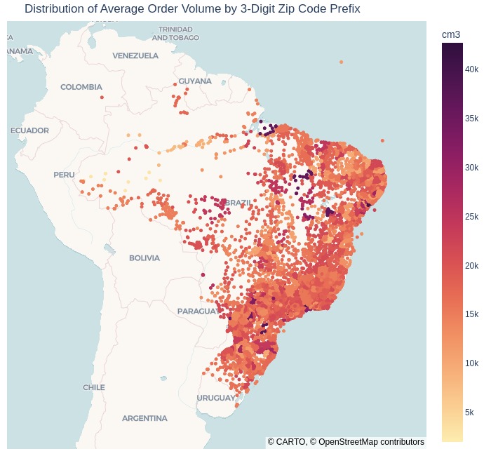
What regions have the largest volume orders?

plot_map_zip('avg_order_volume_cm3')

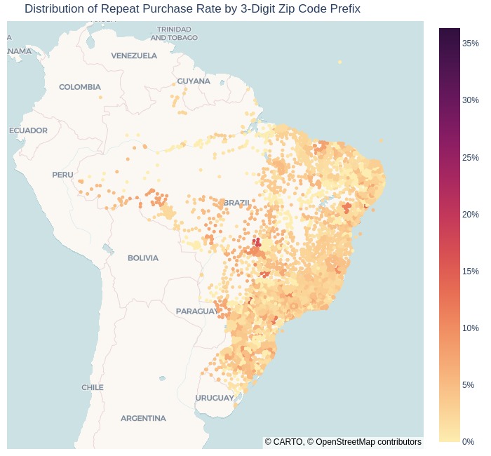
What regions have a higher repeat purchases rate?

plot_map_zip('repeat_purchase_rate')

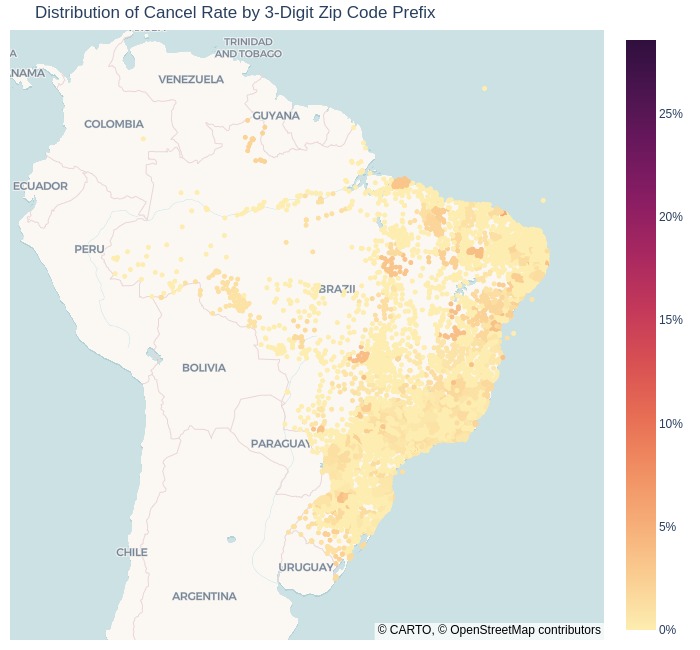
What regions have a higher proportion of canceled orders?

plot_map_zip('cancel_rate')

Geo-analysis by State

Data Preparation

Creating dataframe for visualization

tmp_df_res = (
    df_sales.merge(df_customers_origin[['customer_id', 'customer_state_short', 'population', ]], on='customer_id', how='left')
)
tmp_df_res['is_delayed'] = tmp_df_res['is_delayed'] == 'Delayed'
tmp_df_res['order_has_installment'] = tmp_df_res['order_has_installment'] == 'Has Installments'

Calculate average MAU by state.

temp_mau = (
    tmp_df_res.groupby(['customer_state_short', pd.Grouper(key='order_purchase_dt', freq='ME')], observed=False)
    .agg(mau = ('customer_unique_id', 'nunique'))
    .groupby('customer_state_short', observed=False)
    .mean()
)

tmp_df_res = (
    tmp_df_res.groupby('customer_state_short', observed=False, as_index=False)
    .agg(
        total_orders=('order_id', 'nunique')
        , total_payment = ('total_payment', 'sum')
        , aov = ('total_payment', 'mean')
        , first_orders_cnt = ('sale_is_customer_first_purchase', 'sum')
        , installment_orders_cnt = ('order_has_installment', 'sum')
        , total_reviews = ('reviews_cnt', 'sum')
        , avg_review_score = ('order_avg_reviews_score', 'mean')
        , avg_delivery_time_days = ('delivery_time_days', 'mean')
        , avg_delivery_delay_days = ('delivery_delay_days', 'mean')
        , avg_installments = ('total_installments_cnt', 'mean')
        , avg_products_cnt = ('products_cnt', 'mean')
        , population = ('population', 'first')
        , avg_order_weight_kg = ('total_weight_kg', 'mean')
        , avg_order_volume_cm3 = ('total_volume_cm3', 'mean')
    )
    .merge(temp_mau, on='customer_state_short', how='left')
)

tmp_df_res = (
    df_orders.assign(
        is_canceled = lambda x: x.order_status=='Canceled'
    )
    .merge(df_customers_origin[['customer_id', 'customer_state_short']], on='customer_id')
    .groupby('customer_state_short', as_index=False)
    .agg(
        cancel_rate = ('is_canceled', 'mean')
    )
    .merge(tmp_df_res, on='customer_state_short', how='right')
)

tmp_df_res['orders_per_thousand_person'] = tmp_df_res['total_orders'] * 1000 / tmp_df_res['population']
tmp_df_res['total_payment_per_thousand_person'] = tmp_df_res['total_payment'] * 1000 / tmp_df_res['population']
tmp_df_res['repeat_purchase_rate'] = (tmp_df_res['total_orders'] - tmp_df_res['first_orders_cnt']) / tmp_df_res['total_orders']
tmp_df_res['installment_orders_rate'] = tmp_df_res['installment_orders_cnt'] / tmp_df_res['total_orders']

del temp_mau

Let’s calculate the median retention of the first lifetime by state through cohorts. We will define the period as 30 days.

retention_1st_month_state = (
    df_sales.merge(df_customers_origin[['customer_id', 'customer_state_short']], on='customer_id', how='left')
)

retention_1st_month_state['cohort'] = retention_1st_month_state['customer_first_purchase_dt'].dt.to_period('M')
retention_1st_month_state['lifetime'] = (retention_1st_month_state['order_purchase_dt'] - retention_1st_month_state['customer_first_purchase_dt']).dt.days // 30

retention_1st_month_state = (
    retention_1st_month_state.groupby(['customer_state_short', 'cohort', 'lifetime'])['customer_unique_id']
    .nunique()
    .unstack()
    .fillna(0)
)

retention_1st_month_state = retention_1st_month_state.div(retention_1st_month_state[0], axis=0)[1].reset_index()

retention_1st_month_state = (
    retention_1st_month_state.groupby('customer_state_short', as_index=False, observed=False)
    .median()
)

retention_1st_month_state['retention_1st_month_state'] = retention_1st_month_state[1]

retention_1st_month_state = retention_1st_month_state[['customer_state_short', 'retention_1st_month_state']]

tmp_df_res = tmp_df_res.merge(retention_1st_month_state, on='customer_state_short', how='left')

Data Visualization

Add some metrics in labels_for_map

labels_for_map.update(dict(
    total_reviews = 'Number of Reviews'
    , avg_delivery_delay_days = 'Average Delivery Delay, days'
    , orders_per_thousand_person = 'Number of Orders per Thousand Residents'
    , total_payment_per_thousand_person = 'Sales Amount per Thousand Residents, R$'
    , retention_1st_month_state = 'Retention 1st Month by State'
    , customer_state_short = 'Customer State'
))
labels_for_map.update({'mau': 'Average MAU'})

Let’s calculate the centroids of the states.

brazil_states_geojson = "https://raw.githubusercontent.com/codeforamerica/click_that_hood/master/public/data/brazil-states.geojson"
with urlopen(brazil_states_geojson) as response:
    geojson = json.load(response)

gdf = gpd.GeoDataFrame.from_features(geojson['features'])

gdf['centroid'] = gdf['geometry'].centroid
gdf['centroid_lon'] = gdf['centroid'].x
gdf['centroid_lat'] = gdf['centroid'].y

state_centroids = gdf[['sigla', 'centroid_lon', 'centroid_lat']]
state_centroids.head(1)

	sigla	centroid_lon	centroid_lat
0	AC	-70.44	-9.31

def plot_map_state(metric: str):
    """Create plotly map by states"""
    title = f"Distribution of {labels_for_map[metric].split(',')[0]} by State"
    colorbar_title = labels_for_map[metric].split(',')[1] if ',' in labels_for_map[metric] else None
    df_for_color_text = tmp_df_res[['customer_state_short', metric]]
    color_level = (tmp_df_res[metric].max() - tmp_df_res[metric].min()) * 0.7 + tmp_df_res[metric].min()
    df_for_color_text['color'] = df_for_color_text[metric].apply(lambda x: 'rgba(255, 255, 255, 0.8)'  if x < color_level else 'rgba(50, 50, 50, 0.8)')

    # print(tmp_df_res)
    hover_data = dict()
    is_percentage = metric in [
        'avg_freight_ratio', 'orders_delayed_share', 
        'installment_orders_rate', 'repeat_purchase_rate', 
        'cancel_rate', 'retention_1st_month_state']
    if metric != 'total_orders':
        hover_data['total_orders'] = ':.2s'
    if not is_percentage:
        hover_data[metric] = ':.2s'
    else:
        if metric == 'retention_1st_month_state':
            hover_data[metric] = ':.2%'
        else:
            hover_data[metric] = ':.1%'

    fig = px.choropleth(
        tmp_df_res,
        geojson=brazil_states_geojson,
        locations='customer_state_short',  
        featureidkey="properties.sigla", 
        color=metric,
        color_continuous_scale="Viridis",
        title=title,
        labels=labels_for_map,
        hover_data=hover_data
    )

    fig.add_trace(
        go.Scattergeo(
            lon=state_centroids['centroid_lon'],
            lat=state_centroids['centroid_lat'],
            text=state_centroids['sigla'],
            hoverinfo='none',
            mode='text',
            textfont=dict(
                color='gray',
                size=10
            ),
            showlegend=False
        )
    )

    color_dict = dict(zip(df_for_color_text['customer_state_short'], df_for_color_text['color']))
    for trace in fig.data:
        if trace.type == 'scattergeo':
            states_in_trace = trace.text
            ordered_colors = [color_dict[state] for state in states_in_trace]
            trace.textfont.color = ordered_colors

    if is_percentage:
        fig.update_coloraxes(
            colorbar_tickformat=".0%" if metric != 'retention_1st_month_state' else ".2%"
        )
        
    fig.update_geos(
        visible=False,
        lataxis_range=[-40.7, 7.3],  
        lonaxis_range=[-85, -34.5],  
        projection_scale=1.2,        
        center=dict(lat=-15, lon=-55)  
    )
    
    fig.update_layout(
        margin={"r":0,"t":50,"l":0,"b":0}
        , width=550
        , height=500
        , coloraxis_colorbar_title_text = colorbar_title
    )    
    pb.to_slide(fig)
    return fig

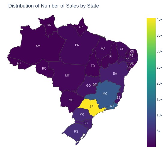
In which states is the sales volume higher?

plot_map_state('total_orders')

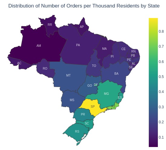
What is the number of orders per resident?

plot_map_state('orders_per_thousand_person')

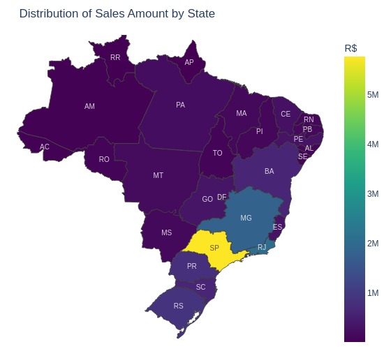
In which states is the sales amount higher?

plot_map_state('total_payment')

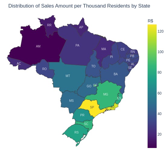
What is the sales amount per resident?

plot_map_state('total_payment_per_thousand_person')

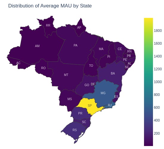
In which states is the average MAU higher?

plot_map_state('mau')

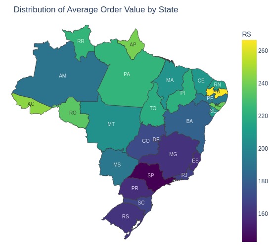
What is the average order value higher in which states?

plot_map_state('aov')

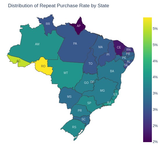
What is the proportion of repeat purchases by states?

plot_map_state('repeat_purchase_rate')

In which states is the number of reviews higher?

plot_map_state('total_reviews')

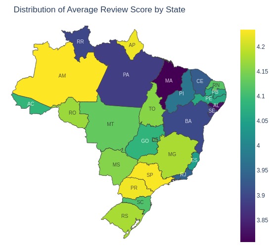
What is the review score higher in which states?

plot_map_state('avg_review_score')

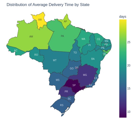
What is the average delivery time higher in which states?

plot_map_state('avg_delivery_time_days')

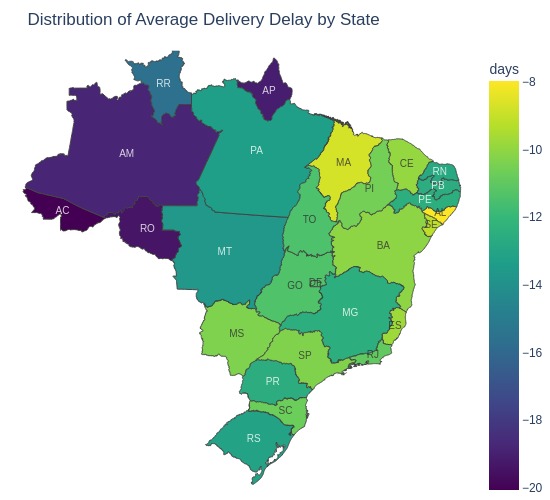
What is the average delivery delay higher in which states?

plot_map_state('avg_delivery_delay_days')

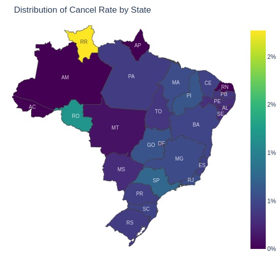
What is the proportion of canceled orders higher in which states?

plot_map_state('cancel_rate')

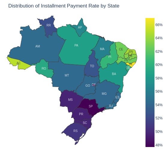
What is the proportion of orders with installment payments higher in which states?

plot_map_state('installment_orders_rate')

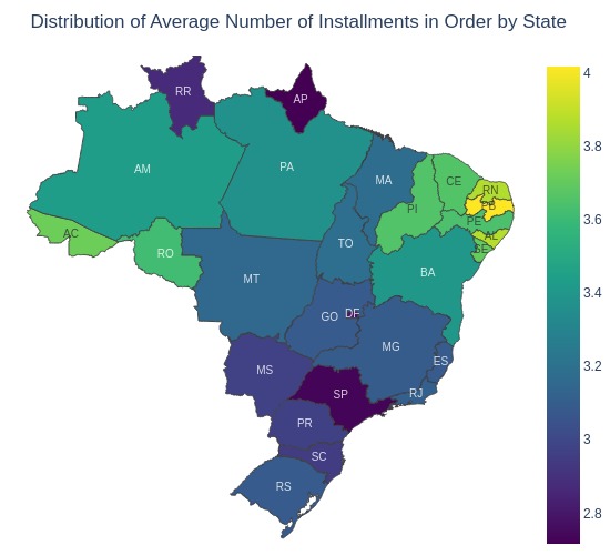
What is the number of installments higher in which states?

plot_map_state('avg_installments')

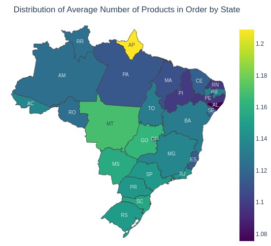
What is the number of items per order higher in which states?

plot_map_state('avg_products_cnt')

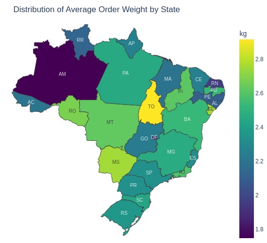
In which states are the heaviest orders?

plot_map_state('avg_order_weight_kg')

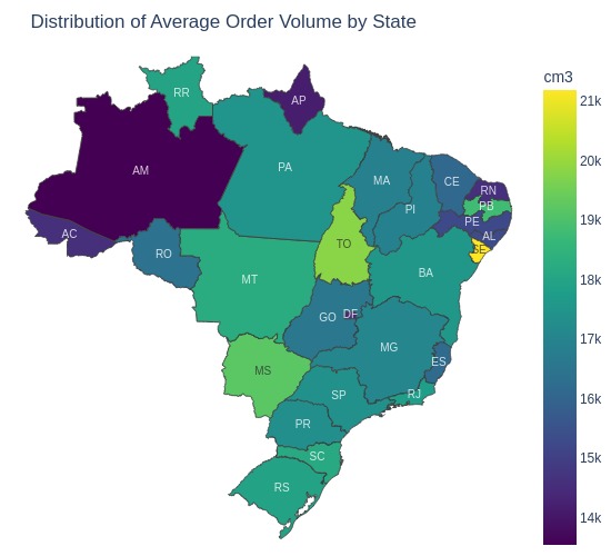
In which states are the largest volume orders?

plot_map_state('avg_order_volume_cm3')

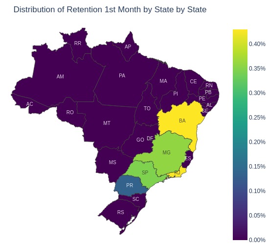
What is the median retention of the first month higher in which states?

plot_map_state('retention_1st_month_state')