Correlation Analysis#
Here we will build a correlation matrix for all numerical variables.
We will also create scatter plots for those with a correlation coefficient greater than 0.3.
Additionally, we can create scatter plots for specific pairs even if the correlation coefficient is low, as we are focused on the relationship rather than the correlation coefficient itself.
Table df_sales#
We will create labels for column names.
labels = {
    'from_purchase_to_approved_hours': 'Purchase To Approved',
    'from_purchase_to_carrier_days': 'Purchase To Carrier',
    'delivery_time_days': 'Delivery Time',
    'delivery_time_estimated_days': 'Estimated Delivery',
    'delivery_delay_days': 'Delivery Delay',
    'from_approved_to_carrier_days': 'Approved To Carrier',
    'from_carrier_to_customer_days': 'Carrier To Customer',
    'payments_cnt': 'Payments Cnt',
    'total_payment': 'Total Payment',
    'avg_payment': 'Avg Payment',
    'total_installments_cnt': 'Total Installments',
    'products_cnt': 'Products Cnt',
    'unique_products_cnt': 'Unique Products Cnt',
    'sellers_cnt': 'Sellers Cnt',
    'product_categories_cnt': 'Categories Cnt',
    'total_products_price': 'Total Products Price',
    'avg_products_price': 'Avg Product Price',
    'total_freight_value': 'Total Freight Value',
    'total_order_price': 'Total Order Price',
    'total_weight_kg': 'Total Weight',
    'total_volume_cm3': 'Total Volume',
    'avg_distance_km': 'Avg Distance',
    'avg_carrier_delivery_delay_days': 'Avg Carrier Delay',
    'freight_ratio': 'Freight Ratio',
    'reviews_cnt': 'Reviews Cnt',
    'order_avg_reviews_score': 'Avg Review Score'
}
Let’s look at the correlation between the metrics.
df_sales.analysis.corr_matrix(labels=labels)
/home/pagri/.cache/pypoetry/virtualenvs/olist-deep-dive-kC-yxADm-py3.13/lib/python3.13/site-packages/frameon/dataframe/analysis/correlation.py:283: ConstantInputWarning:

An input array is constant; the correlation coefficient is not defined.
/home/pagri/.cache/pypoetry/virtualenvs/olist-deep-dive-kC-yxADm-py3.13/lib/python3.13/site-packages/frameon/dataframe/analysis/correlation.py:283: ConstantInputWarning:

An input array is constant; the correlation coefficient is not defined.
/home/pagri/.cache/pypoetry/virtualenvs/olist-deep-dive-kC-yxADm-py3.13/lib/python3.13/site-packages/frameon/dataframe/analysis/correlation.py:283: ConstantInputWarning:

An input array is constant; the correlation coefficient is not defined.
/home/pagri/.cache/pypoetry/virtualenvs/olist-deep-dive-kC-yxADm-py3.13/lib/python3.13/site-packages/frameon/dataframe/analysis/correlation.py:283: ConstantInputWarning:

An input array is constant; the correlation coefficient is not defined.
/home/pagri/.cache/pypoetry/virtualenvs/olist-deep-dive-kC-yxADm-py3.13/lib/python3.13/site-packages/frameon/dataframe/analysis/correlation.py:283: ConstantInputWarning:

An input array is constant; the correlation coefficient is not defined.
/home/pagri/.cache/pypoetry/virtualenvs/olist-deep-dive-kC-yxADm-py3.13/lib/python3.13/site-packages/frameon/dataframe/analysis/correlation.py:283: ConstantInputWarning:

An input array is constant; the correlation coefficient is not defined.
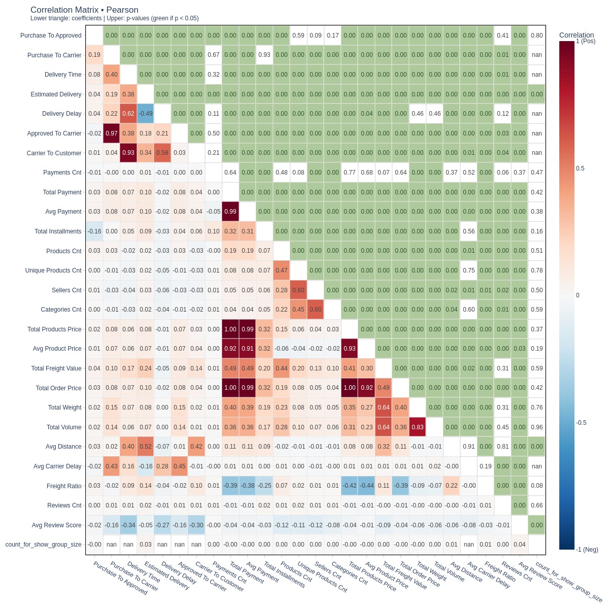
Key Observations:
There is a moderate positive correlation (0.4) between the total delivery time and the delivery time to the carrier. Therefore, the delivery time to the carrier affects the total delivery time, which is logical.
There is a moderate positive correlation (0.6) between the total delivery time and the delivery time from the carrier. The delivery time from the carrier has a higher correlation with the total delivery time compared to the delivery time to the carrier. This suggests that the delivery time from the carrier affects the total delivery time more significantly.
There is a moderate positive correlation (0.5) between the total number of products in an order and the number of unique products in an order. This indicates that the total number of products in an order often increases due to the addition of unique products rather than by increasing the quantity of already existing products in the order.
There is also a moderate positive correlation (0.6) between the number of sellers in an order and the number of unique products in an order. This means that if customers buy more unique products, they are likely to buy from different sellers.
There is also a moderate positive correlation (0.6) between the number of sellers in an order and the number of categories in an order. This indicates that if customers buy products from more categories, they are likely to buy from different sellers.
There is a moderate positive correlation (0.5) between the delivery cost of an order and the order amount. This means that the more expensive the order, the higher the delivery cost, which is logical.
There is a moderate positive correlation (0.6) between the delivery cost of an order and the weight/volume of the order. This suggests that the heavier or larger the order, the higher the delivery cost.
There is a strong positive correlation (0.8) between the volume and weight of the order. This indicates that the heavier the order, the larger it is usually.
Does the order cost affect the delivery cost?
df_sales.viz.pairplot(
    pairs=['total_payment', 'total_freight_value']
    , transforms='log'
    , labels=labels
)
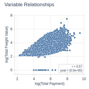
Key Observations:
Higher order value → higher shipping cost
Does the order weight affect the delivery cost?
df_sales.viz.pairplot(
    pairs=['total_weight_kg', 'total_freight_value']
    , transforms='log'
    , labels=labels
)
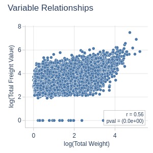
Key Observations:
Heavier orders → higher shipping cost
Does the order volume affect the delivery cost?
df_sales.viz.pairplot(
    pairs=['total_volume_cm3', 'total_freight_value']
    , transforms='log'
    , labels=labels
)
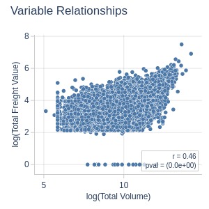
Key Observations:
Larger volume → higher shipping cost
Does the distance affect the delivery cost?
df_sales.viz.pairplot(
    pairs=['avg_distance_km', 'total_freight_value']
    , transforms='log'
    , labels=labels
)
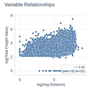
Key Observations:
Greater distance → higher shipping cost
Does the order cost affect the delivery time?
df_sales.viz.pairplot(
    pairs=['total_payment', 'delivery_time_days']
    , transforms='log'
    , labels=labels
)
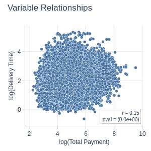
Key Observations:
Order value has minimal impact on delivery time
Does the order weight affect the delivery time?
df_sales.viz.pairplot(
    pairs=['total_weight_kg', 'delivery_time_days']
    , transforms='log'
    , labels=labels
)
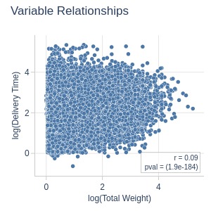
Key Observations:
Weight has minimal impact on delivery time
Does the order volume affect the delivery time?
df_sales.viz.pairplot(
    pairs=['total_volume_cm3', 'delivery_time_days']
    , transforms='log'
    , labels=labels
)
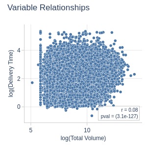
Key Observations:
Volume doesn’t affect delivery time
Does the distance affect the delivery time?
df_sales.viz.pairplot(
    pairs=['avg_distance_km', 'delivery_time_days']
    , transforms='log'
    , labels=labels
)
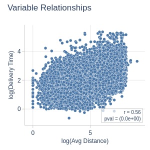
Key Observations:
Greater distance → longer delivery time
Is the heavier the order, the larger its volume?
df_sales.viz.pairplot(
    pairs=['total_weight_kg', 'total_volume_cm3']
    , transforms='log'
    , labels=labels
)
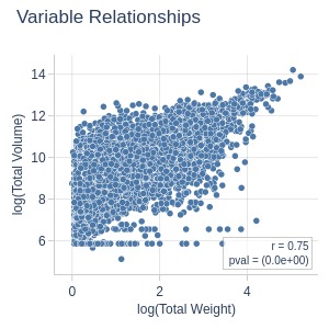
Key Observations:
Heavier items tend to be larger
Table df_customers#
We will create labels for column names.
labels = {
    'orders_cnt': 'Total Orders',
    'canceled_share': 'Canceled Share',
    'canceled_orders_cnt': 'Canceled Orders',
    'not_delivered_share': 'Not Delivered Share',
    'customer_issue_share': 'Customer Issue Share',
    'service_issue_share': 'Service Issue Share',
    'buys_cnt': 'Total Purchases',
    'avg_delivery_time_days': 'Avg Delivery Time',
    'avg_delivery_delay_days': 'Avg Delivery Delay',
    'delayed_orders_share': 'Delayed Orders Share',
    'purchase_weekend_share': 'Weekend Purchase Share',
    'repeat_purchase_share': 'Repeat Purchase Share',
    'avg_payments_cnt': 'Avg Payments Cnt',
    'total_customer_payment': 'Total Payment',
    'avg_total_order_payment': 'Avg Order Payment',
    'avg_individual_payment': 'Avg Individual Payment',
    'installment_orders_share': 'Installment Orders Share',
    'avg_products_cnt': 'Avg Products Cnt',
    'avg_unique_products_cnt': 'Avg Unique Products',
    'avg_sellers_cnt': 'Avg Sellers Cnt',
    'avg_order_total_products_price': 'Avg Order Products Price',
    'avg_total_order_price': 'Avg Total Order Price',
    'avg_products_price': 'Avg Product Price',
    'total_products_price': 'Total Products Price',
    'avg_order_total_freight_value': 'Avg Order Freight Value',
    'avg_order_total_weight_kg': 'Avg Order Weight',
    'avg_order_total_volume_cm3': 'Avg Order Volume',
    'free_shipping_share': 'Free Shipping Share',
    'reviews_cnt': 'Reviews Cnt',
    'customer_avg_reviews_score': 'Avg Review Score',
    'avg_distance_km': 'Avg Distance',
    'avg_buys_diff_days': 'Days Between Purchases',
    'months_with_buys': 'Active Months',
    'max_consecutive_months_with_buys': 'Max Consecutive Active Months'
}
Let’s look at the correlation between the metrics.
exclude_cols = ['lat_customer', 'lng_customer', 'customer_zip_code_prefix_3_digits', 'population', 'customer_zip_code_prefix']
(
    df_customers.drop(columns=exclude_cols)
    .analysis.corr_matrix(text_size=10, labels=labels)
)
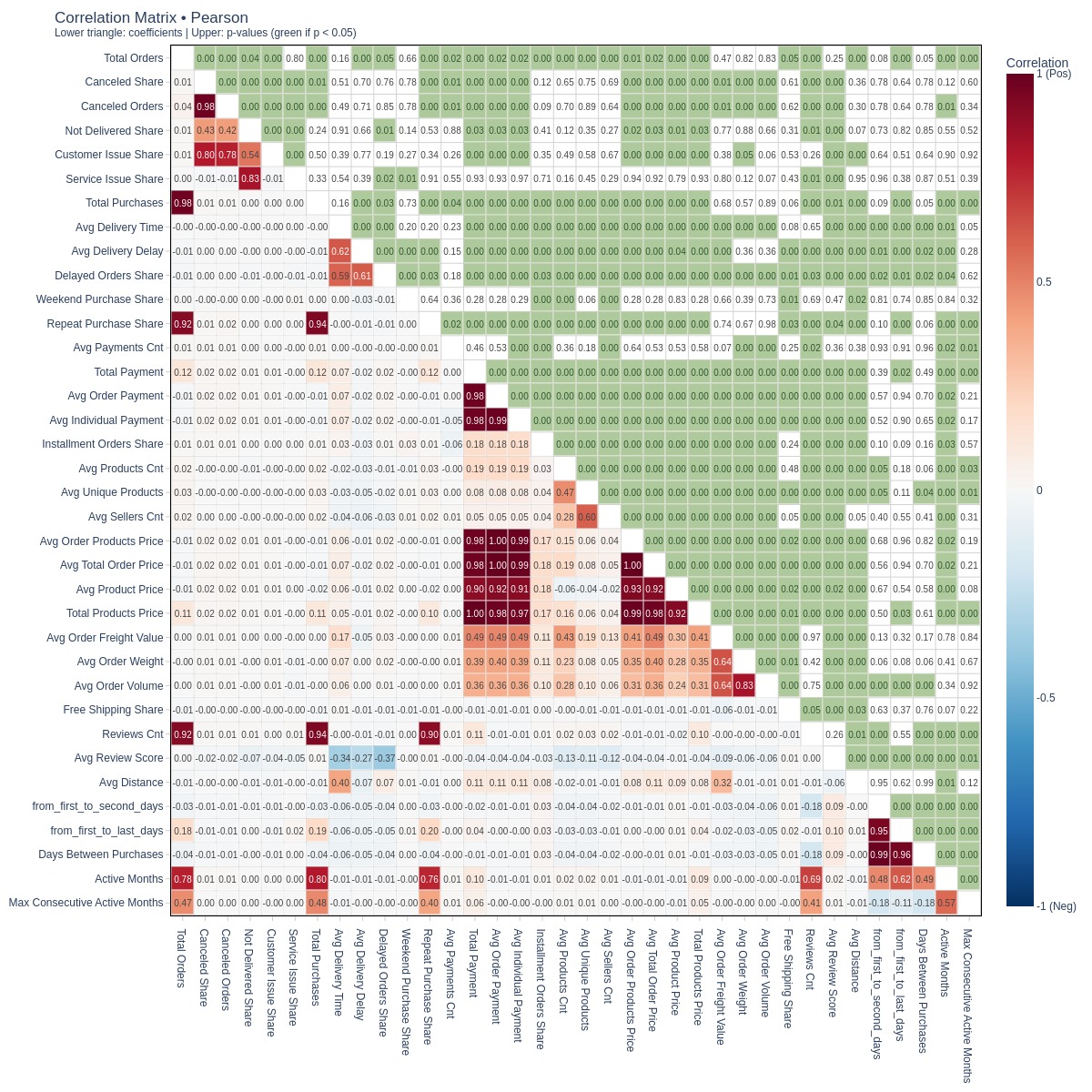
Key Observations:
There is a high positive correlation (0.8) between the number of canceled orders and the proportion of issues due to the customer. This is logical, as the Canceled status is included in the proportion of customer issues.
There is a high positive correlation (0.9) between the number of orders and the number of reviews. Therefore, the more orders a customer makes, the more reviews they leave.
Are there “loyal” customers with high activity?
df_customers.viz.pairplot(
    pairs=['max_consecutive_months_with_buys', 'orders_cnt']
    , labels=labels
)
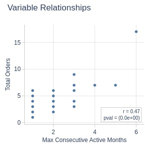
Key Observations:
More active months → more orders
If customers buy many unique products, are the orders from different sellers?
df_customers.viz.pairplot(
    pairs=['avg_unique_products_cnt', 'avg_sellers_cnt']
    , transforms='log'
    , labels=labels
)
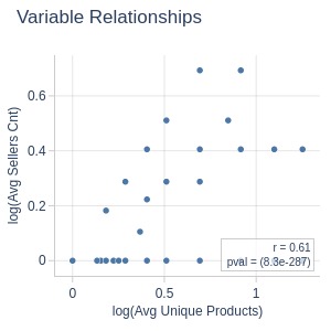
Key Observations:
The higher the average number of unique products in an order for a customer, the higher the average number of sellers. This means that different products are more often bought from different sellers.
Are active customers more likely to write reviews?
df_customers.viz.pairplot(
    pairs=['reviews_cnt', 'orders_cnt']
    , transforms='log'
    , labels=labels
)
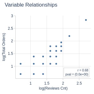
Key Observations:
More purchases → more reviews left