Product Analysis

Number of Products

pb.configure(
    df = df_products
    , metric = 'product_sales_cnt'
    , metric_label = 'Share of Sold Products'
    , agg_func = 'sum'
    , norm_by='all'
    , axis_sort_order='descending'
    , text_auto='.1%'
    , update_fig={'xaxis': {'tickformat': '.0%'}}
)

print(f'Total sold products count: {df_products.product_sales_cnt.sum():,.0f}')

Total sold products count: 100,051

Let’s look at the top values of the metrics

pb.metric_top(id_column='product_id')

	product_sales_cnt
product_id
99a4788cb24856965c36a24e339b6058	456.00
aca2eb7d00ea1a7b8ebd4e68314663af	425.00
422879e10f46682990de24d770e7f83d	352.00
d1c427060a0f73f6b889a5c7c61f2ac4	313.00
389d119b48cf3043d311335e499d9c6b	309.00
53b36df67ebb7c41585e8d54d6772e08	304.00
368c6c730842d78016ad823897a372db	291.00
53759a2ecddad2bb87a079a1f1519f73	287.00
154e7e31ebfa092203795c972e5804a6	262.00
2b4609f8948be18874494203496bc318	254.00

Let’s see at statistics and distribution of the metric.

pb.metric_info(
    labels=dict(product_sales_cnt='Number of Units Sold per Product')
    , title='Distribution of Number of Units Sold per Product'
    , upper_quantile=0.99
    , hist_mode='dual_hist_trim'
)

Summary Statistics for "product_sales_cnt" (Type: Integer)

Summary			Percentiles			Detailed Stats			Value Counts
Total	32.12k (97%)		Max	456		Mean	3.11		1	19.05k (58%)
Missing	829 (3%)		99%	30		Trimmed Mean (10%)	1.68		2	5.30k (16%)
Distinct	124 (<1%)		95%	10		Mode	1		3	2.34k (7%)
Non-Duplicate	38 (<1%)		75%	2		Range	455		4	1.31k (4%)
Duplicates	32.83k (99%)		50%	1		IQR	1		5	882 (3%)
Dup. Values	86 (<1%)		25%	1		Std	9.43		6	576 (2%)
Zeros	---		5%	1		MAD	0		7	450 (1%)
Negative	---		1%	1		Kurt	622.35		8	311 (<1%)
Memory Usage	<1 Mb		Min	1		Skew	19.93		9	252 (<1%)

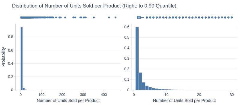
Key Observations:

• 75% of products sold 1-2 units total

• Top 5% sold ≥10 units

Let’s look at the statistics and distribution of the number of sold products per day.

tmp_df_res = (
    df_sales.merge(df_items, on='order_id', how='left')
    .groupby(pd.Grouper(key='order_purchase_dt', freq='D'), observed=False)['product_id']
    .nunique()
    .to_frame('products_cnt_per_day')
)

tmp_df_res['products_cnt_per_day'].explore.info(
    labels=dict(orders_cnt_per_day='Number of Sold Products per Day')
    , title='Distribution of Number of Sold Products per Day'
)

Summary Statistics for "products_cnt_per_day" (Type: Integer)

Summary			Percentiles			Detailed Stats			Value Counts
Total	602 (100%)		Max	901		Mean	153.55		150	7 (1%)
Missing	---		99%	333.93		Trimmed Mean (10%)	150.00		239	7 (1%)
Distinct	258 (43%)		95%	276.95		Mode	Multiple		98	6 (<1%)
Non-Duplicate	101 (17%)		75%	206.75		Range	897		67	6 (<1%)
Duplicates	344 (57%)		50%	143.50		IQR	108.75		141	6 (<1%)
Dup. Values	157 (26%)		25%	98		Std	79.36		66	6 (<1%)
Zeros	---		5%	45.10		MAD	76.35		192	6 (<1%)
Negative	---		1%	8.03		Kurt	12.14		103	6 (<1%)
Memory Usage	<1 Mb		Min	4		Skew	1.62		102	6 (<1%)

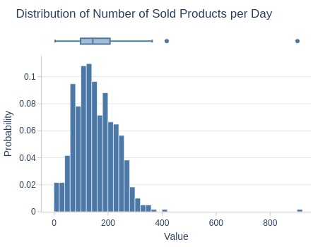
Key Observations:

• 75% of days sold ≤207 products

• Top 5% sold ≥277 products

• Several days exceeded 400 products

Let’s look by different dimensions.

By Product Category

fig = pb.bar_groupby(
    y='product_category'
    , trim_top_n_y=20
    , width=1100
    , height=500   
    , show_top_and_bottom_n = 15
    , show_count=False
).update_layout(xaxis_domain=[0, 0.4], xaxis2_domain=[0.6, 1], xaxis2_tickformat='.2%')
pb.to_slide(fig)
fig.show()

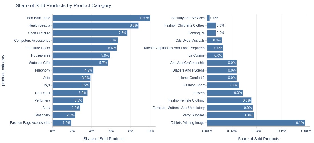
Key Observations:

• Best-selling categories: Bed Bath Table, Health Beauty

• Lowest-selling: Security and Services

By Generalized Product Category

pb.bar_groupby(y='general_product_category', to_slide=True)

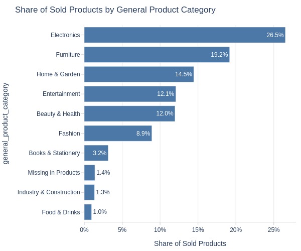
Key Observations:

• Top 3 generalized categories by units sold:

  1. Electronics (27%)

  2. Furniture (19%)

  3. Home & Garden (15%)

• Lowest: Food & Drinks (1%)

Product Price

pb.configure(
    df = df_products
    , metric = 'avg_price'
    , metric_label = 'Average Product Price, R$'
    , metric_label_for_distribution = 'Product Price, R$'
    , agg_func = 'mean'
    , axis_sort_order='descending'
    , text_auto='.3s'
)

Top products.

pb.metric_top(id_column='product_id')

	avg_price
product_id
489ae2aa008f021502940f251d4cce7f	6,735.00
69c590f7ffc7bf8db97190b6cb6ed62e	6,729.00
1bdf5e6731585cf01aa8169c7028d6ad	6,499.00
a6492cc69376c469ab6f61d8f44de961	4,799.00
c3ed642d592594bb648ff4a04cee2747	4,690.00
259037a6a41845e455183f89c5035f18	4,590.00
a1beef8f3992dbd4cd8726796aa69c53	4,399.87
6cdf8fc1d741c76586d8b6b15e9eef30	4,099.99
6902c1962dd19d540807d0ab8fade5c6	3,999.90
4ca7b91a31637bd24fb8e559d5e015e4	3,999.00

Let’s see at statistics and distribution of the metric.

pb.metric_info(
    labels=dict(product_sales_cnt='Average Product Price, R$')
    , title='Distribution of Average Product Price'
    , upper_quantile=0.99
    , hist_mode='dual_hist_trim'
)

Summary Statistics for "avg_price" (Type: Float)

Summary			Percentiles			Detailed Stats			Value Counts
Total	32.12k (97%)		Max	6.74k		Mean	144.59		59.90	508 (2%)
Missing	829 (3%)		99%	1.20k		Trimmed Mean (10%)	96.88		39.90	387 (1%)
Distinct	8.64k (26%)		95%	469.90		Mode	59.90		69.90	378 (1%)
Non-Duplicate	6.35k (19%)		75%	153.33		Range	6.73k		49.90	363 (1%)
Duplicates	24.31k (74%)		50%	79		IQR	113.43		19.90	320 (<1%)
Dup. Values	2.29k (7%)		25%	39.90		Std	247.00		29.90	319 (<1%)
Zeros	---		5%	16.90		MAD	71.16		89.90	274 (<1%)
Negative	---		1%	9.82		Kurt	103.20		79.90	256 (<1%)
Memory Usage	<1 Mb		Min	0.85		Skew	7.62		99.90	252 (<1%)

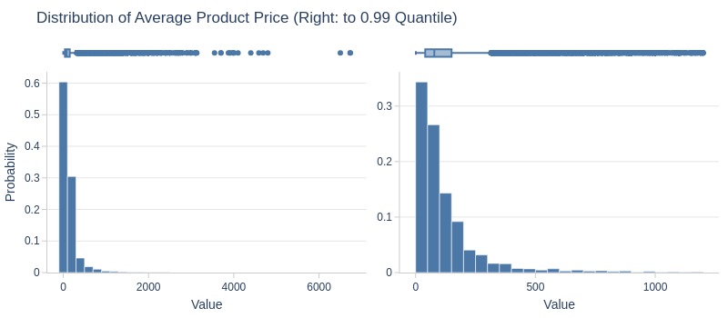
Key Observations:

• 75% of products had average price ≤153 R$

• Bottom 5% ≤17 R$

• Top 5% ≥470 R$

Let’s see at statistics and distribution of the metric per day.

tmp_df_res = (
    df_sales.merge(df_items, on='order_id', how='left')
    .groupby(pd.Grouper(key='order_purchase_dt', freq='D'), observed=False)['price']
    .mean()
    .to_frame('avg_price_per_day')
)

tmp_df_res['avg_price_per_day'].explore.info(
    labels=dict(avg_price_per_day='Average Product Price per Day, R$')
    , title='Distribution of Average Product Price per Day, R$'
)

Summary Statistics for "avg_price_per_day" (Type: Float)

Summary			Percentiles			Detailed Stats			Value Counts
Total	602 (100%)		Max	270.38		Mean	121.70		12.40	1 (<1%)
Missing	---		99%	229.02		Trimmed Mean (10%)	118.95		108.33	1 (<1%)
Distinct	602 (100%)		95%	162.41		Mode	Multiple		113.69	1 (<1%)
Non-Duplicate	602 (100%)		75%	129.87		Range	257.98		110.72	1 (<1%)
Duplicates	---		50%	117.27		IQR	21.90		108.30	1 (<1%)
Dup. Values	---		25%	107.97		Std	24.95		135.27	1 (<1%)
Zeros	---		5%	93.56		MAD	16.13		106.63	1 (<1%)
Negative	---		1%	81.65		Kurt	8.41		120.96	1 (<1%)
Memory Usage	<1 Mb		Min	12.40		Skew	1.96		93.40	1 (<1%)

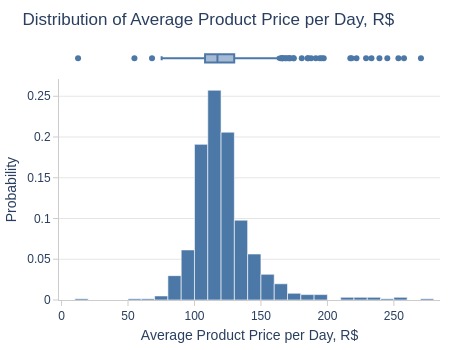
Key Observations:

• Daily average product prices:

  • Bottom 5% ≤94 R$

  • Middle 50% 108-130 R$

  • Top 5% ≥162 R$

Let’s look by different dimensions.

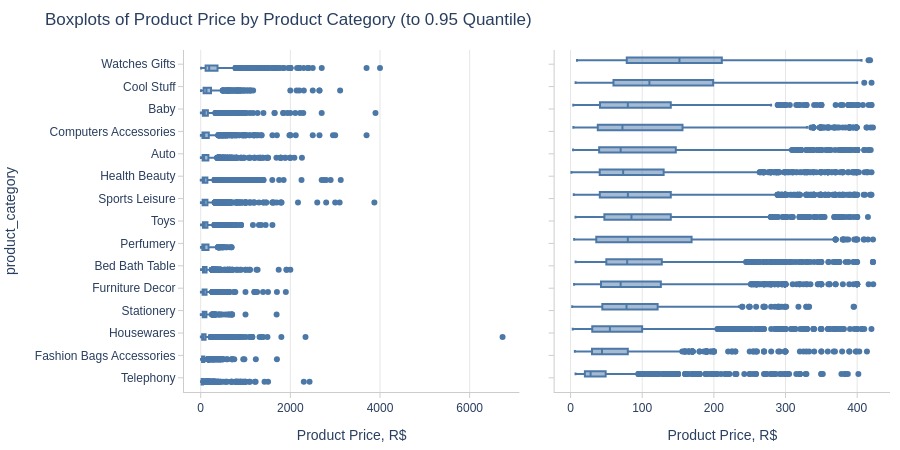
By Product Category

print('Top Best')
pb.box(y='product_category').show()
print('Top Worst')
pb.box(
    y='product_category'
    , trim_top_n_direction='bottom'
).show()
pb.bar_groupby(
    y='product_category'
    , show_top_and_bottom_n=15
    , to_slide=True
).show()

Top Best

Top Worst

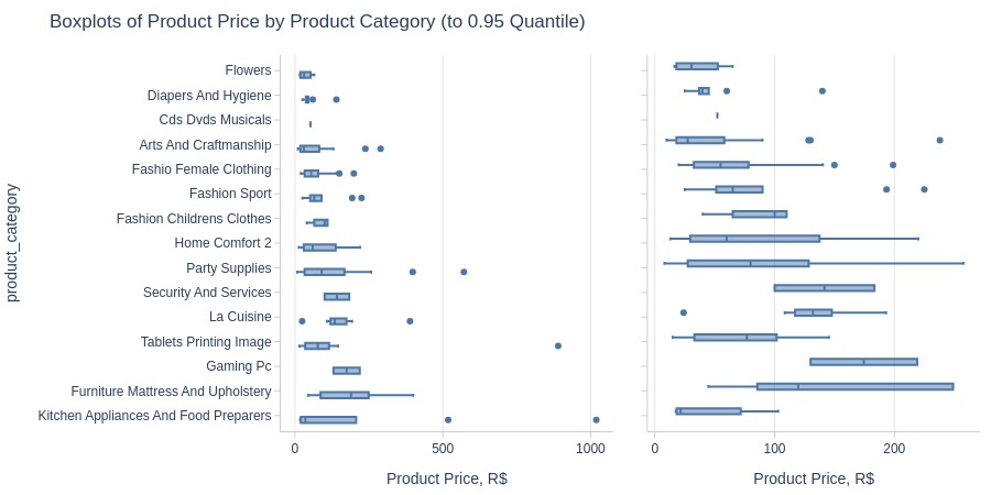
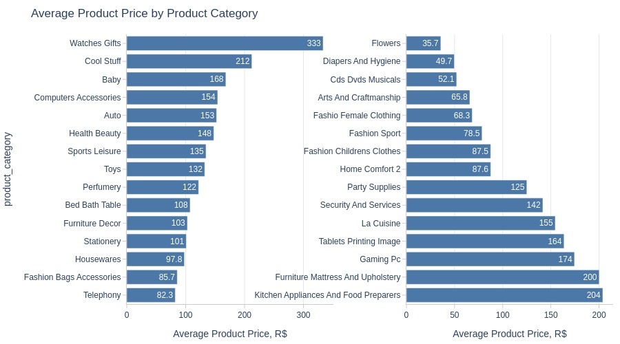
Key Observations:

• Highest priced category: Watches Gifts

• Lowest priced: Flowers

By Generalized Product Category

pb.box(y='general_product_category').show()
fig = pb.bar_groupby(
    y='general_product_category'
    , show_count=True
).update_layout(xaxis2_title_text='Number of Sold Products')
pb.to_slide(fig)
fig.show()

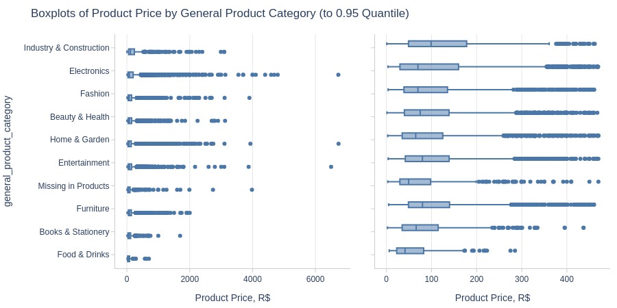
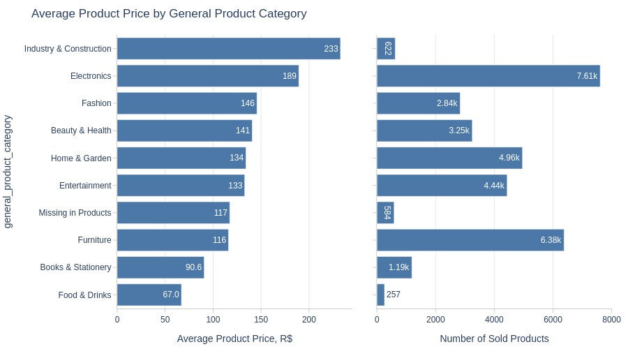
Key Observations:

• Top 3 categories by average price:

  1. Industry & Construction

  2. Electronics

  3. Fashion

• Lowest: Food & Drinks

Sales Amount of Products

pb.configure(
    df = df_products
    , metric = 'total_sales_amount'
    , metric_label = 'Total Sales Amount of Products, R$'
    , metric_label_for_distribution = 'Total Sales Amount per Product, R$'
    , agg_func = 'sum'
    , axis_sort_order='descending'
    , text_auto='.3s'
)

Top products.

pb.metric_top(id_column='product_id')

	total_sales_amount
product_id
bb50f2e236e5eea0100680137654686c	63,560.00
6cdd53843498f92890544667809f1595	53,652.30
d6160fb7873f184099d9bc95e30376af	45,949.35
d1c427060a0f73f6b889a5c7c61f2ac4	45,620.56
99a4788cb24856965c36a24e339b6058	42,049.66
3dd2a17168ec895c781a9191c1e95ad7	40,782.80
25c38557cf793876c5abdd5931f922db	38,907.32
5f504b3a1c75b73d6151be81eb05bdc9	37,733.90
53b36df67ebb7c41585e8d54d6772e08	37,454.63
aca2eb7d00ea1a7b8ebd4e68314663af	37,104.30

Let’s see at statistics and distribution of the metric per day.

tmp_df_res = (
    df_sales.merge(df_items, on='order_id', how='left')
    .groupby(pd.Grouper(key='order_purchase_dt', freq='D'), observed=False)['price']
    .sum()
    .to_frame('total_price_per_day')
)

tmp_df_res['total_price_per_day'].explore.info(
    labels=dict(avg_price_per_day='Total Product Price per Day, R$')
    , title='Distribution of Total Product Price per Day, R$'
)

Summary Statistics for "total_price_per_day" (Type: Float)

Summary			Percentiles			Detailed Stats			Value Counts
Total	602 (100%)		Max	149.92k		Mean	21.93k		396.90	1 (<1%)
Missing	---		99%	49.69k		Trimmed Mean (10%)	21.20k		23507.49	1 (<1%)
Distinct	602 (100%)		95%	41.51k		Mode	Multiple		33539.34	1 (<1%)
Non-Duplicate	602 (100%)		75%	28.81k		Range	149.52k		30891.45	1 (<1%)
Duplicates	---		50%	20.34k		IQR	15.82k		27074.86	1 (<1%)
Dup. Values	---		25%	12.99k		Std	12.23k		30571.07	1 (<1%)
Zeros	---		5%	5.83k		MAD	11.60k		20579.17	1 (<1%)
Negative	---		1%	1.44k		Kurt	18.99		22014.31	1 (<1%)
Memory Usage	<1 Mb		Min	396.90		Skew	2.20		23255.73	1 (<1%)

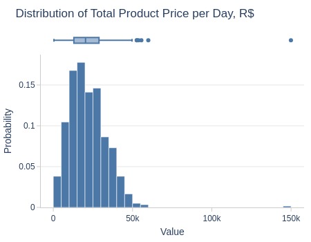
Key Observations:

• 75% of days had product revenue ≤29K R$

• Top 5% ≥42K R$

Let’s look by different dimensions.

By Product Category

print('Top Best')
pb.box(y='product_category').show()
print('Top Worst')
pb.box(
    y='product_category'
    , trim_top_n_direction='bottom'
).show()
pb.bar_groupby(
    y='product_category'
    , show_top_and_bottom_n=15
    , horizontal_spacing=0.25
    , to_slide=True
).show()

Top Best

Top Worst

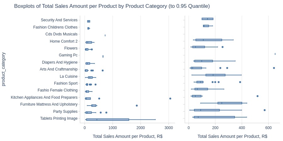
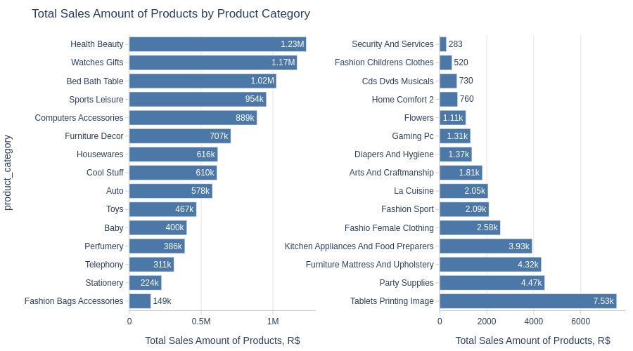
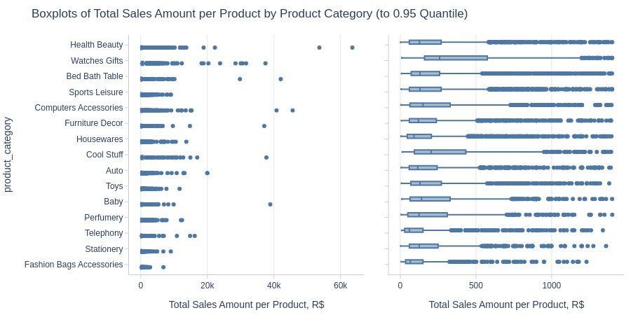
Key Observations:

• Highest revenue categories: Health beauty, Watches gifts

• Lowest: Security and services

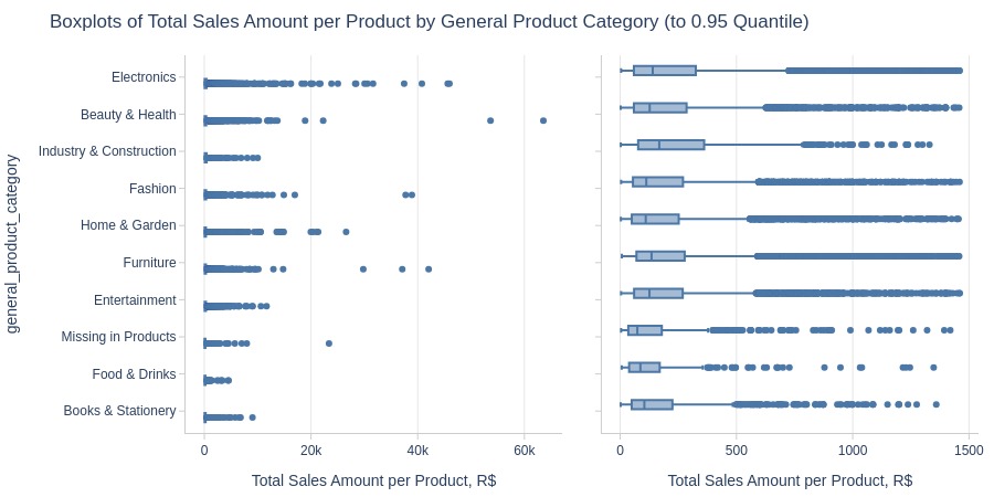
By Generalized Product Category

pb.box(y='general_product_category').show()
fig = (
    pb.bar_groupby(y='general_product_category', show_count=True)
    .update_layout(
        xaxis2_title_text='Number of Sold Products'
    )
)
pb.to_slide(fig)
fig.show()

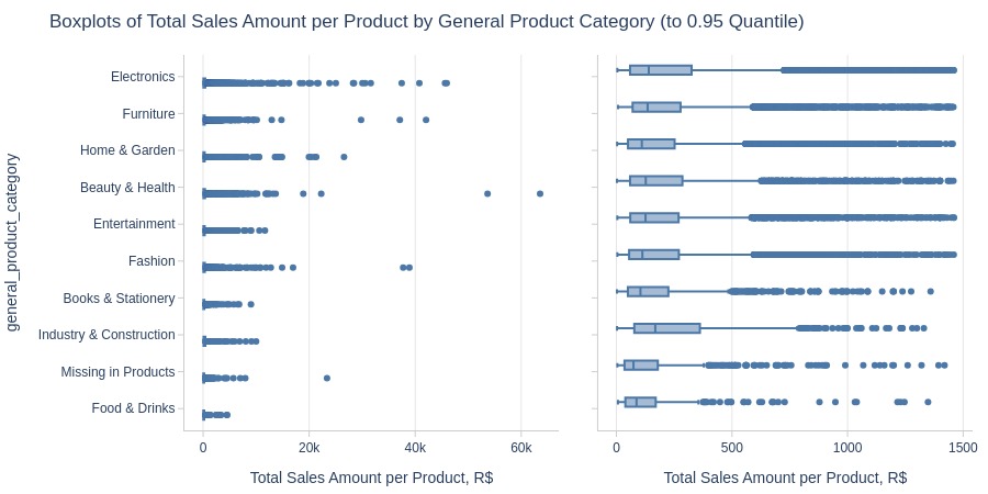
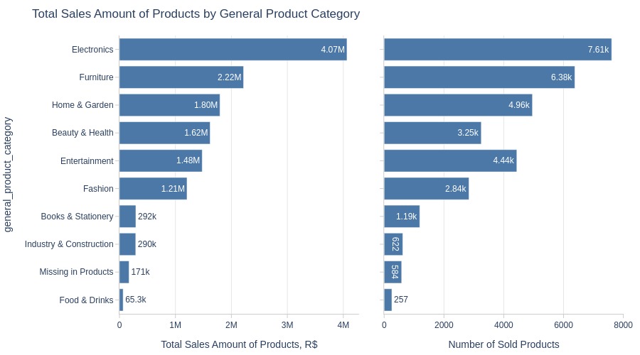
Key Observations:

• Top 3 categories by revenue:

  1. Electronics

  2. Furniture

  3. Home & Garden

• Lowest: Food & Drinks

Sales Amount per Product

pb.configure(
    df = df_products
    , metric = 'total_sales_amount'
    , metric_label = 'Average Sales Amount per Products, R$'
    , metric_label_for_distribution = 'Total Sales Amount per Product, R$'
    , agg_func = 'mean'
    , axis_sort_order='descending'
    , text_auto='.3s'    
)

Let’s see at statistics and distribution of the metric.

pb.metric_info(
    labels=dict(total_sales_amount='Total Sales Amount per Product, R$')
    , title='Distribution of Total Sales Amount per Product'
    , upper_quantile=0.99
    , hist_mode='dual_hist_trim'
)

Summary Statistics for "total_sales_amount" (Type: Float)

Summary			Percentiles			Detailed Stats			Value Counts
Total	32.12k (97%)		Max	63.56k		Mean	410.98		59.90	363 (1%)
Missing	829 (3%)		99%	4.69k		Trimmed Mean (10%)	198.54		69.90	251 (<1%)
Distinct	10.14k (31%)		95%	1.46k		Mode	59.90		39.90	245 (<1%)
Non-Duplicate	7.12k (22%)		75%	325.88		Range	63.56k		49.90	219 (<1%)
Duplicates	22.81k (69%)		50%	135.99		IQR	265.98		29.90	218 (<1%)
Dup. Values	3.02k (9%)		25%	59.90		Std	1.36k		89.90	200 (<1%)
Zeros	---		5%	20.03		MAD	138.61		19.90	195 (<1%)
Negative	---		1%	11.57		Kurt	499.53		79.90	173 (<1%)
Memory Usage	<1 Mb		Min	2.20		Skew	17.70		99.90	171 (<1%)

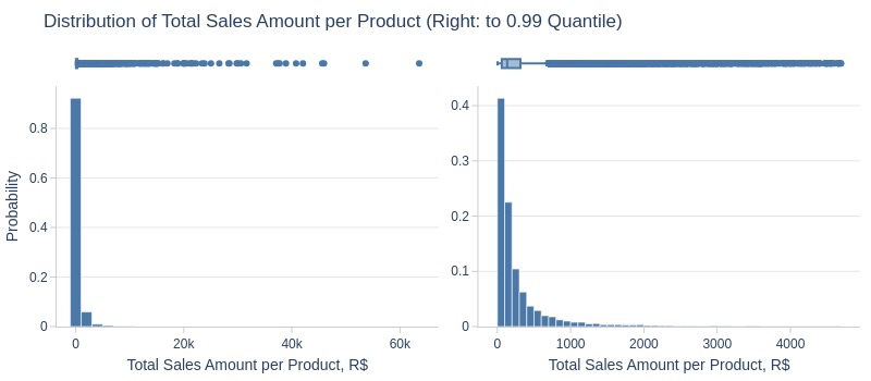
Key Observations:

• 75% of products generated ≤325 R$ lifetime revenue

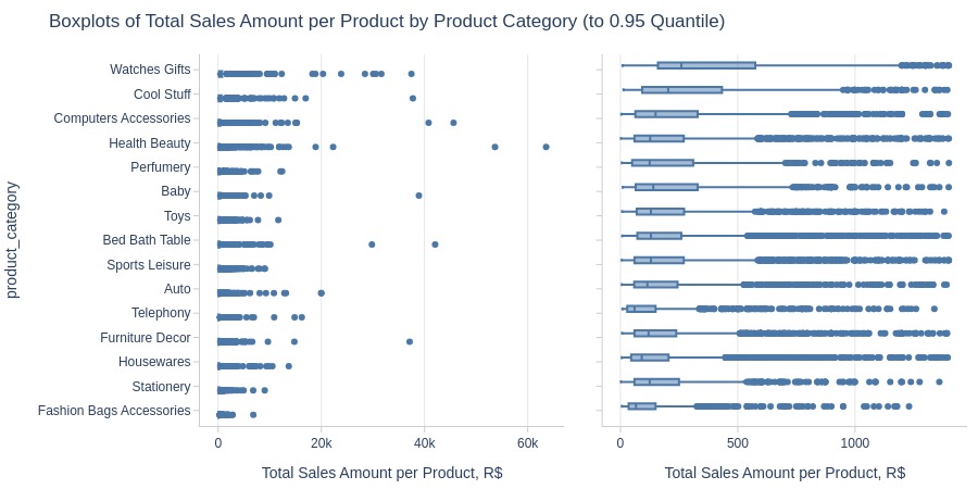
Let’s look by different dimensions.

By Product Category

print('Top Best')
pb.box(y='product_category').show()
print('Top Worst')
pb.box(
    y='product_category'
    , trim_top_n_direction='bottom'
).show()
pb.bar_groupby(
    y='product_category'
    , show_top_and_bottom_n=15
    , horizontal_spacing=0.25
    , to_slide=True
)

Top Best

Top Worst

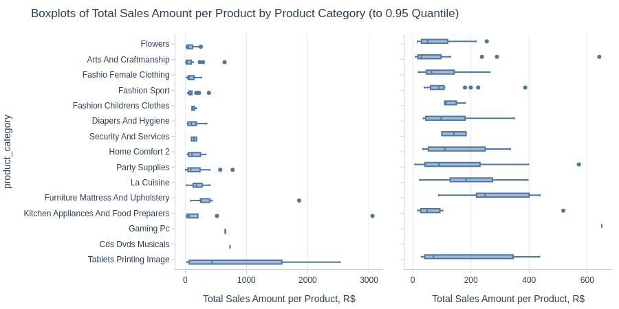
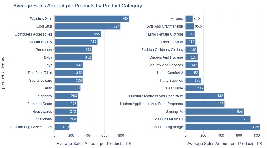
Key Observations:

• Highest average revenue per product: Watches gifts

• Lowest: Flowers

By Generalized Product Category

pb.box(y='general_product_category').show()
pb.bar_groupby(y='general_product_category', to_slide=True).show()

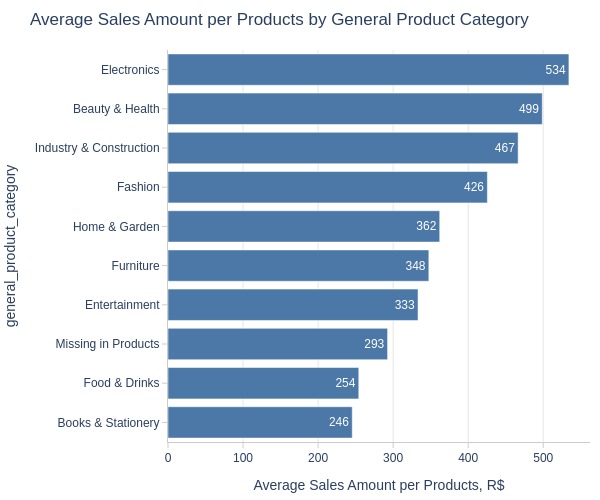
Key Observations:

• Top 3 categories by average revenue:

  1. Electronics

  2. Beauty & Health

  3. Industry & Construction

• Lowest: Books & Stationery

Price Range

pb.configure(
    df = df_products
    , metric = 'price_range'
    , metric_label = 'Average Price Range per Product, R$'
    , metric_label_for_distribution = 'Price Range per Product, R$'
    , agg_func = 'mean'
    , axis_sort_order='descending'
    , text_auto='.2f'
)

Top products.

pb.metric_top(id_column='product_id')

	price_range
product_id
8b502ca34e28d30605bc667b965b6abf	999.10
5237739bb5fee495dbd337755a138660	740.00
ba16581014183c8415da15145f3d4c24	660.99
a7c87b1bbdd51e0d68b0307cffd03d47	650.01
18209df52bc87a69b84db4df602397c1	519.01
68f3adaef1620e7b0c4c7cd9f78d7ed0	497.35
4cce3fa9fee9eb2361e0b9bd32516958	461.00
d6160fb7873f184099d9bc95e30376af	449.99
f819f0c84a64f02d3a5606ca95edd272	400.09
c1afa44a5a60e2e7cf7280e57eba0597	400.00

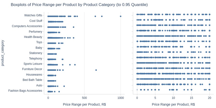
Let’s see at statistics and distribution of the metric.

pb.metric_info(
    upper_quantile=0.95
    , hist_mode='dual_hist_trim'
)

Summary Statistics for "price_range" (Type: Float)

Summary			Percentiles			Detailed Stats			Value Counts
Total	32.12k (97%)		Max	999.10		Mean	3.94		0	26.35k (80%)
Missing	829 (3%)		99%	70.01		Trimmed Mean (10%)	0.44		10	518 (2%)
Distinct	1.83k (6%)		95%	20		Mode	0		20	235 (<1%)
Non-Duplicate	1.29k (4%)		75%	0		Range	999.10		5	230 (<1%)
Duplicates	31.12k (94%)		50%	0		IQR	0		1	153 (<1%)
Dup. Values	536 (2%)		25%	0		Std	19.74		4	150 (<1%)
Zeros	26.35k (80%)		5%	0		MAD	0		2	141 (<1%)
Negative	---		1%	0		Kurt	465.73		3	128 (<1%)
Memory Usage	<1 Mb		Min	0		Skew	16.31		6	120 (<1%)

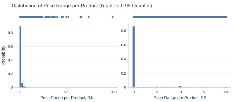
Key Observations:

• 80% of products maintained stable prices

• 5% had price changes ≥20 R$

Let’s look by different dimensions.

By Product Category

print('Top Best')
pb.box(y='product_category').show()
print('Top Worst')
pb.box(
    y='product_category'
    , trim_top_n_direction='bottom'
).show()
pb.bar_groupby(
    y='product_category'
    , show_top_and_bottom_n=15
    , horizontal_spacing=0.25
    , to_slide=True
).show()

Top Best

Top Worst

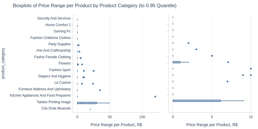
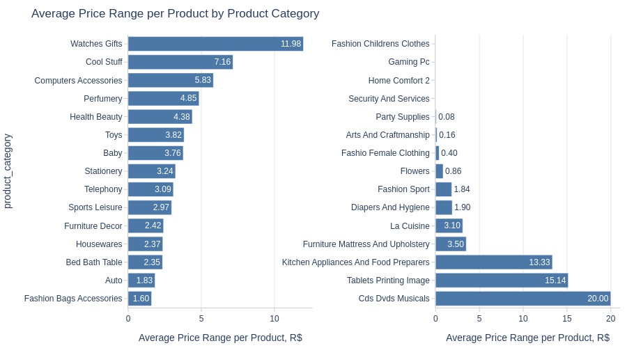
Key Observations:

• Most price volatility: Watches gifts

By Generalized Product Category

pb.box(y='general_product_category').show()
pb.bar_groupby(y='general_product_category', to_slide=True)

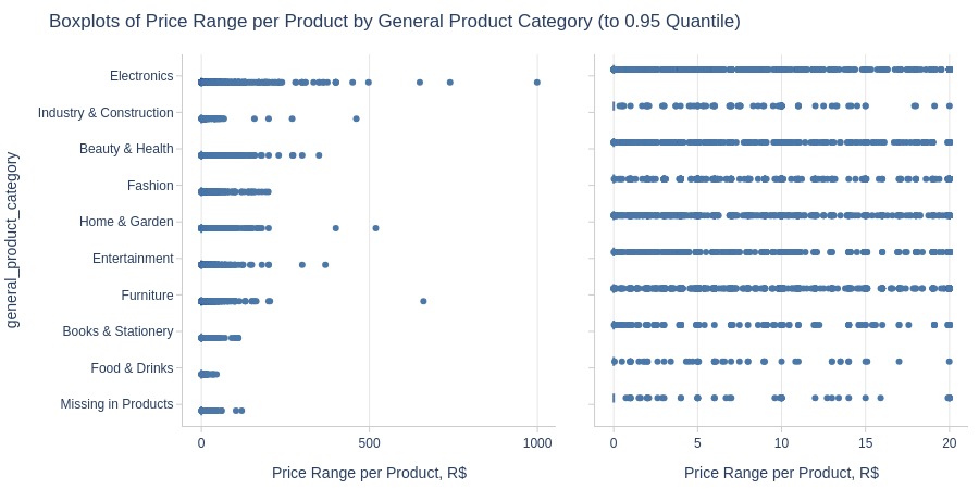
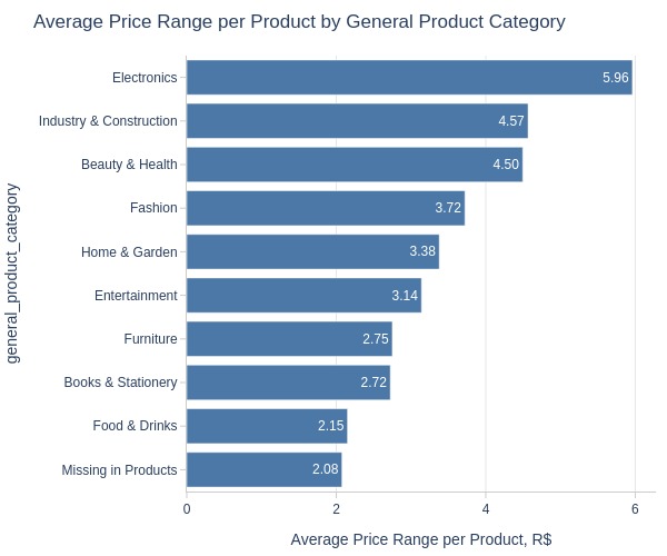
Key Observations:

• Top 3 categories by price changes:

  1. Electronics

  2. Industry & Construction

  3. Beauty & Health

• Lowest volatility: Food & Drinks

Quantity of Product per Order

pb.configure(
    df = df_products
    , metric = 'avg_product_qty_per_order'
    , metric_label = 'Average Quantity of Product per Order'
    , agg_func = 'mean'
    , axis_sort_order='descending'
    , text_auto='.3s'
)

Top products.

pb.metric_top(id_column='product_id')

	avg_product_qty_per_order
product_id
9571759451b1d780ee7c15012ea109d4	20.00
37eb69aca8718e843d897aa7b82f462d	15.00
05b515fdc76e888aada3c6d66c201dff	10.00
270516a3f41dc035aa87d220228f844c	10.00
89b190a046022486c635022524a974a8	10.00
5769ef0a239114ac3a854af00df129e4	8.00
810cfa5dd36b001cfc186499381f72ab	7.00
4cce2fad3d2dec6f82510d2521aebdd3	7.00
ce6184189a523c1eb5fe5113061780b9	6.00
ac1ad58efc1ebf66bfadc09f29bdedc0	6.00

Let’s see at statistics and distribution of the metric.

pb.metric_info(
    upper_quantile=0.95
    , hist_mode='dual_hist_trim'
)

Summary Statistics for "avg_product_qty_per_order" (Type: Float)

Summary			Percentiles			Detailed Stats			Value Counts
Total	32.12k (97%)		Max	20		Mean	1.11		1	27.88k (85%)
Missing	829 (3%)		99%	3		Trimmed Mean (10%)	1.00		2	1.22k (4%)
Distinct	305 (<1%)		95%	2		Mode	1		1.50	534 (2%)
Non-Duplicate	175 (<1%)		75%	1		Range	19		1.33	254 (<1%)
Duplicates	32.65k (99%)		50%	1		IQR	0		3	203 (<1%)
Dup. Values	130 (<1%)		25%	1		Std	0.45		1.25	182 (<1%)
Zeros	---		5%	1		MAD	0		1.20	156 (<1%)
Negative	---		1%	1		Kurt	188.05		1.17	104 (<1%)
Memory Usage	<1 Mb		Min	1		Skew	9.45		4	101 (<1%)

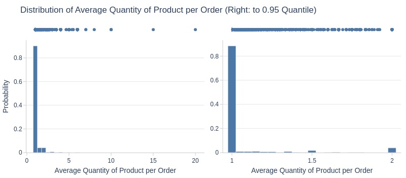
Key Observations:

• 85% of products appeared as single units in orders

Let’s look by different dimensions.

By Generalized Product Category

pb.box(y='general_product_category').show()
pb.bar_groupby(y='general_product_category').show()

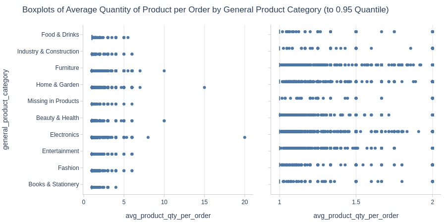
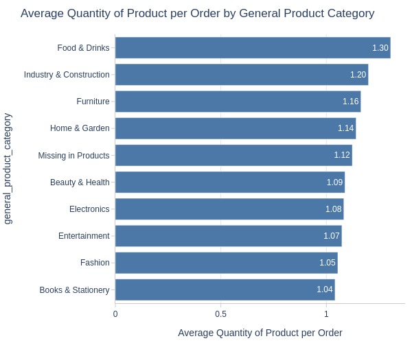
Key Observations:

• Highest average quantity per order: Food & Drinks

Length of Product Name

pb.configure(
    df = df_products
    , metric = 'product_name_lenght'
    , metric_label = 'Length of Product Name'
)

Top products.

pb.metric_top(id_column='product_id')

	product_name_lenght
product_id
aac3cc525702d53c8a2f4733ed214098	76.00
52b3af7304d611855714d9b3d1724ea7	72.00
2e2b9bfa91068239d5fb2b39764b92a5	69.00
2b19dbb6e225fc04cf9a80d83f949b88	68.00
df6e62772d439c7afc2d284339cf9425	67.00
023a60ac6b3484afe23d788ce2444df0	66.00
3ed31fdf8af68a6c0b059a256420a5c5	64.00
33041fc111e526d9dd16e06678ff5eeb	64.00
81a5ad77c14cd83d0c853e4c317cb837	64.00
05a6b99c0460f22f5f8101493c0e3c0e	64.00

Let’s see at statistics and distribution of the metric.

pb.metric_info()

Summary Statistics for "product_name_lenght" (Type: Integer)

Summary			Percentiles			Detailed Stats			Value Counts
Total	32.34k (98%)		Max	76		Mean	48.48		60	2.18k (7%)
Missing	610 (2%)		99%	63		Trimmed Mean (10%)	49.63		59	2.02k (6%)
Distinct	66 (<1%)		95%	60		Mode	60		58	1.89k (6%)
Non-Duplicate	7 (<1%)		75%	57		Range	71		57	1.72k (5%)
Duplicates	32.88k (99%)		50%	51		IQR	15		55	1.68k (5%)
Dup. Values	59 (<1%)		25%	42		Std	10.25		56	1.68k (5%)
Zeros	---		5%	29		MAD	10.38		54	1.44k (4%)
Negative	---		1%	20		Kurt	0.19		53	1.33k (4%)
Memory Usage	<1 Mb		Min	5		Skew	-0.90		52	1.26k (4%)

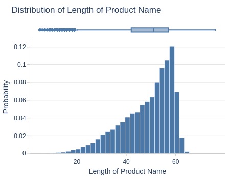
Key Observations:

• 75% of products have names ≤57 characters

Length of Product Description

pb.configure(
    df = df_products
    , metric = 'product_description_lenght'
    , metric_label = 'Length of Product Description'
)

Top products.

pb.metric_top(id_column='product_id')

	product_description_lenght
product_id
47d52bb24ef8a3aa09724f00604be3ba	3,992.00
e6f1f7e12ef3f7c254164e35be6420db	3,988.00
84fad62439091ff986a3885bfd6d299d	3,985.00
ddebc97ddf43a9787d1ee7012e394ccc	3,976.00
7a40001d3da620600ab80109510f3496	3,963.00
c6d339a1fa8873b1ffe76fb1b7cc10f1	3,956.00
1bdf5e6731585cf01aa8169c7028d6ad	3,954.00
cd8c7501d1e3a66f282dfed8dbd5ab9f	3,954.00
ed43976cb61c922803515e4963d9e5cc	3,950.00
8a90417eb713be09fd87a5d077ae06a2	3,949.00

Let’s see at statistics and distribution of the metric.

pb.metric_info()

Summary Statistics for "product_description_lenght" (Type: Integer)

Summary			Percentiles			Detailed Stats			Value Counts
Total	32.34k (98%)		Max	3.99k		Mean	771.50		404	94 (<1%)
Missing	610 (2%)		99%	3.29k		Trimmed Mean (10%)	662.91		729	86 (<1%)
Distinct	2.96k (9%)		95%	2.06k		Mode	404		651	66 (<1%)
Non-Duplicate	669 (2%)		75%	972		Range	3.99k		703	66 (<1%)
Duplicates	29.99k (91%)		50%	595		IQR	633		236	65 (<1%)
Dup. Values	2.29k (7%)		25%	339		Std	635.12		184	65 (<1%)
Zeros	---		5%	150		MAD	434.40		303	63 (<1%)
Negative	---		1%	84		Kurt	4.83		352	62 (<1%)
Memory Usage	<1 Mb		Min	4		Skew	1.96		375	60 (<1%)

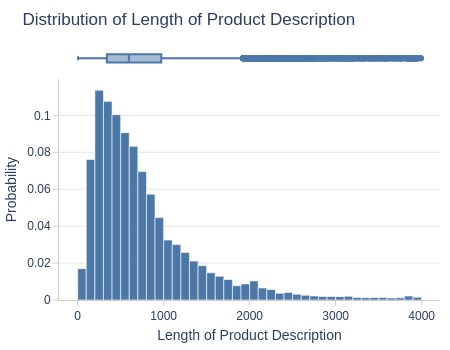
Key Observations:

• 75% of products have descriptions ≤1000 characters

Number of Product Photos

pb.configure(
    df = df_products
    , metric = 'product_photos_qty'
    , metric_label = 'Number of Product Photos'
)

Top products.

pb.metric_top(id_column='product_id')

	product_photos_qty
product_id
f95d5d21561ea085ba1e1a4e53840844	20
234495ab7809d4517bc1330c439da1bb	19
e9880042522806f124fdd4f8c8514d0d	18
b659034bc6cfc3d9baeda101c0c281fe	18
f9aa001a859b11fd798bb386f3d07eb0	17
801f0a5ea1ac28df44d65195cf4e2620	17
7f38cf4e517ec6bb1d31c4e6b6df18ef	17
5948868c402a614a2dd3b90ebb06a253	17
b085d8c8840e8dd3d6ccdf3d86c6145e	17
28763a4fd1b597a9c4f31a9579e7d1b4	17

Let’s see at statistics and distribution of the metric.

pb.metric_info()

Summary Statistics for "product_photos_qty" (Type: Integer)

Summary			Percentiles			Detailed Stats			Value Counts
Total	32.95k (100%)		Max	20		Mean	2.17		1	17.10k (52%)
Missing	---		99%	8		Trimmed Mean (10%)	1.81		2	6.26k (19%)
Distinct	19 (<1%)		95%	6		Mode	1		3	3.86k (12%)
Non-Duplicate	2 (<1%)		75%	3		Range	19		4	2.43k (7%)
Duplicates	32.93k (99%)		50%	1		IQR	2		5	1.48k (5%)
Dup. Values	17 (<1%)		25%	1		Std	1.73		6	968 (3%)
Zeros	---		5%	1		MAD	0		7	343 (1%)
Negative	---		1%	1		Kurt	7.39		8	192 (<1%)
Memory Usage	<1 Mb		Min	1		Skew	2.22		9	105 (<1%)

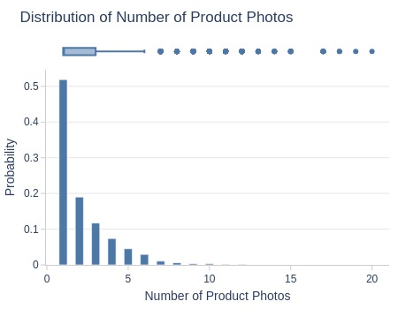
Key Observations:

• 52% of products have 1 photo

• Top 5% have ≥6 photos

Product Weight

pb.configure(
    df = df_products
    , metric = 'product_weight_g'
    , metric_label = 'Product Weight, g'
)

Top products.

pb.metric_top(id_column='product_id')

	product_weight_g
product_id
26644690fde745fc4654719c3904e1db	40425
07f7c5fe95aa4a3b8ea56a5119546939	30000
0e9dfb804bafa3d68ef3ee7a621abfb2	30000
bad9cd5ad615c0b5ba87448e03ec954c	30000
9dfef86fb34051388a7263a31642386c	30000
46e24ce614899e36617e37ea1e4aa6ff	30000
f97ad9066c718a6cef93dfcf253d3e0d	30000
b575098a6da9b81384a7df56314b7f70	30000
cb26d15d1b6eabaac7c0803774245884	30000
0a859d8dc68f6a746b4709217110c439	30000

Let’s see at statistics and distribution of the metric.

pb.metric_info(
    upper_quantile=0.95
    , hist_mode='dual_hist_trim'    
)

Summary Statistics for "product_weight_g" (Type: Integer)

Summary			Percentiles			Detailed Stats			Value Counts
Total	32.95k (100%)		Max	40.42k		Mean	2.28k		200	2.08k (6%)
Missing	---		99%	22.54k		Trimmed Mean (10%)	1.20k		300	1.56k (5%)
Distinct	2.20k (7%)		95%	10.85k		Mode	200		150	1.26k (4%)
Non-Duplicate	1.03k (3%)		75%	1.90k		Range	40423		400	1.21k (4%)
Duplicates	30.75k (93%)		50%	700		IQR	1.60k		100	1.19k (4%)
Dup. Values	1.17k (4%)		25%	300		Std	4.28k		500	1.11k (3%)
Zeros	---		5%	107		MAD	741.30		250	1.00k (3%)
Negative	---		1%	62		Kurt	15.14		600	957 (3%)
Memory Usage	<1 Mb		Min	2		Skew	3.61		350	832 (3%)

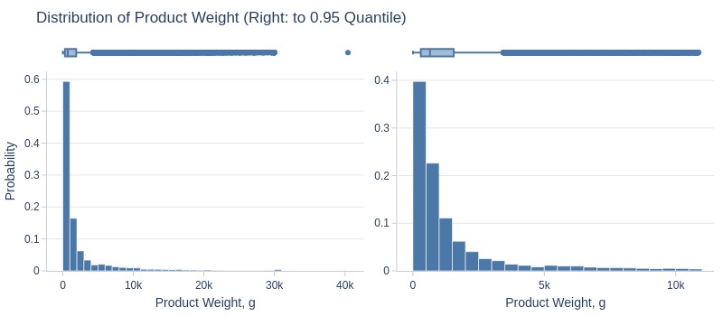
Key Observations:

• 75% of products weigh ≤1.9kg

• Top 5% weigh ≥11kg

Product Length

pb.configure(
    df = df_products
    , metric = 'product_length_cm'
    , metric_label = 'Product Length, cm'
)

Top products.

pb.metric_top(id_column='product_id')

	product_length_cm
product_id
ca8abbdcac2d082a56ff54df35aec76a	105
e10c5041c0752194622a7a7016d8c9b5	105
199f076c011ea5e8b546bff05d4f2477	105
e1717ed4c8d10ca8117e64019d6cb0d0	105
34742604f6cd1e891726b849b6890f81	105
2a9e3d335bbb23ffee8c9da6cecb7bb8	105
032e8352e7d34cc2558d4ae22132866c	105
60dfe129ad287ca8cd2656a8151138ad	105
5ea241885816f6957dfaa9a8592c6b37	105
b33e45187a97dab72b3c819e76efc972	105

Let’s see at statistics and distribution of the metric.

pb.metric_info()

Summary Statistics for "product_length_cm" (Type: Integer)

Summary			Percentiles			Detailed Stats			Value Counts
Total	32.95k (100%)		Max	105		Mean	30.81		16	5.52k (17%)
Missing	---		99%	100		Trimmed Mean (10%)	27.79		20	2.82k (9%)
Distinct	99 (<1%)		95%	65		Mode	16		30	2.03k (6%)
Non-Duplicate	1 (<1%)		75%	38		Range	98		18	1.50k (5%)
Duplicates	32.85k (99%)		50%	25		IQR	20		25	1.39k (4%)
Dup. Values	98 (<1%)		25%	18		Std	16.91		17	1.31k (4%)
Zeros	---		5%	16		MAD	11.86		19	1.27k (4%)
Negative	---		1%	16		Kurt	3.51		40	1.22k (4%)
Memory Usage	<1 Mb		Min	7		Skew	1.75		22	972 (3%)

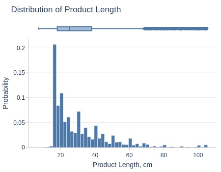
Key Observations:

• 75% of products are ≤38cm long

• Top 5% ≥65cm

Product Width

pb.configure(
    df = df_products
    , metric = 'product_width_cm'
    , metric_label = 'Product Width, cm'
)

Top products.

pb.metric_top(id_column='product_id')

	product_width_cm
product_id
b17808303e15dd50538c011b44295427	118
6d30e5e702df2b8719d9c6be1bdf425b	105
3b17f6528c9e2a01b2f75f844a60ddae	105
a2f4e28e50f60566eeb99f842ffc0fd9	105
cb428376d66b5e216d2ef9f3b27fc172	105
3758055ab2434bd36ac78e00b15b5cf6	105
83d68ad4e5707409089afff26a40b2df	104
e7248872169a7ab67e20c182aaf17976	103
e54c0428a8cf1b79f63823b92e20aacc	102
68e6e8fd8c5f5b252b105d00daa9b57b	102

Let’s see at statistics and distribution of the metric.

pb.metric_info()

Summary Statistics for "product_width_cm" (Type: Integer)

Summary			Percentiles			Detailed Stats			Value Counts
Total	32.95k (100%)		Max	118		Mean	23.20		11	3.72k (11%)
Missing	---		99%	63		Trimmed Mean (10%)	21.39		20	3.05k (9%)
Distinct	95 (<1%)		95%	47		Mode	11		16	2.81k (9%)
Non-Duplicate	9 (<1%)		75%	30		Range	112		15	2.39k (7%)
Duplicates	32.86k (99%)		50%	20		IQR	15		30	1.79k (5%)
Dup. Values	86 (<1%)		25%	15		Std	12.08		12	1.54k (5%)
Zeros	---		5%	11		MAD	8.90		25	1.33k (4%)
Negative	---		1%	11		Kurt	4.07		14	1.26k (4%)
Memory Usage	<1 Mb		Min	6		Skew	1.67		13	1.13k (3%)

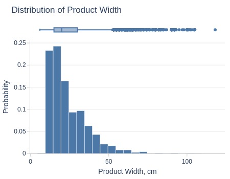
Key Observations:

• 75% of products are ≤30cm wide

• Top 5% ≥47cm

Product Height

pb.configure(
    df = df_products
    , metric = 'product_height_cm'
    , metric_label = 'Product Height, cm'
)

Top products.

pb.metric_top(id_column='product_id')

	product_height_cm
product_id
bc3c6d2a621414f2e1df7a8a32a2828e	105
d14495a85be157b5cacef4eaaf825791	105
1ca99da10c4b800de39096631ed2e773	105
995a6110a2705a9401669fb4cf939241	105
011967a30ceeaa86acb72e79664544ad	105
83f6e0a993efdfa2bf9550a204422cb7	105
e42ad1ff7ad0843110435858ec10a2c6	105
a7f4ab2b8fc3ee762e05b6eda08acb93	105
65b183dcbb9689b176730d709a0003dd	105
e940125d0a3c309f58f41cd21e39af06	105

Let’s see at statistics and distribution of the metric.

pb.metric_info()

Summary Statistics for "product_height_cm" (Type: Integer)

Summary			Percentiles			Detailed Stats			Value Counts
Total	32.95k (100%)		Max	105		Mean	16.94		10	2.55k (8%)
Missing	---		99%	69		Trimmed Mean (10%)	14.74		15	2.02k (6%)
Distinct	102 (<1%)		95%	44		Mode	10		20	1.99k (6%)
Non-Duplicate	3 (<1%)		75%	21		Range	103		16	1.60k (5%)
Duplicates	32.85k (99%)		50%	13		IQR	13		11	1.55k (5%)
Dup. Values	99 (<1%)		25%	8		Std	13.64		5	1.53k (5%)
Zeros	---		5%	3		MAD	8.90		12	1.52k (5%)
Negative	---		1%	2		Kurt	6.68		8	1.47k (4%)
Memory Usage	<1 Mb		Min	2		Skew	2.14		2	1.36k (4%)

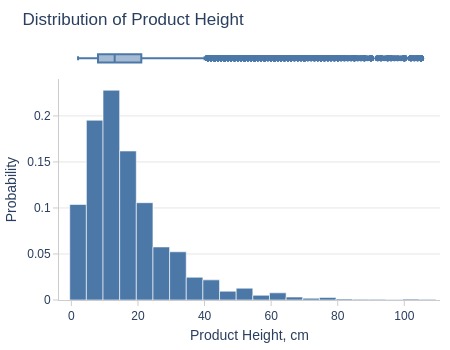
Key Observations:

• 75% of products are ≤21cm tall

• Top 5% ≥44cm

Product Volume

pb.configure(
    df = df_products
    , metric = 'product_volume_cm3'
    , metric_label = 'Product Volume, cm3'
)

Top products.

pb.metric_top(id_column='product_id')

	product_volume_cm3
product_id
256a9c364b75753b97bee410c9491ad8	296,208.00
3eb14e65e4208c6d94b7a32e41add538	294,000.00
0b48eade13cfad433122f23739a66898	294,000.00
c1e0531cb1864fd3a0cae57dca55ca80	294,000.00
f227e2d44f10f7dad30fb4dfa839e7a2	294,000.00
90c1b4e040d1d1c45897ec2dad4a809d	293,706.00
8d6f2c3454002d3f5aa7479a7fad7794	288,000.00
99ff40856c47a638df807c0a144470cc	288,000.00
c6fdec160d0f8f488d9041316c85051d	288,000.00
0e9dfb804bafa3d68ef3ee7a621abfb2	287,980.00

Let’s see at statistics and distribution of the metric.

pb.metric_info()

Summary Statistics for "product_volume_cm3" (Type: Integer)

Summary			Percentiles			Detailed Stats			Value Counts
Total	32.95k (100%)		Max	296.21k		Mean	16.56k		8000	604 (2%)
Missing	---		99%	135.91k		Trimmed Mean (10%)	10.58k		352	588 (2%)
Distinct	4.53k (14%)		95%	63.37k		Mode	8.00k		4096	419 (1%)
Non-Duplicate	1.98k (6%)		75%	18.48k		Range	296.04k		2560	327 (<1%)
Duplicates	28.43k (86%)		50%	6.84k		IQR	15.60k		27000	327 (<1%)
Dup. Values	2.54k (8%)		25%	2.88k		Std	27.06k		23625	259 (<1%)
Zeros	---		5%	832		MAD	7.37k		12000	256 (<1%)
Negative	---		1%	352		Kurt	24.62		1936	239 (<1%)
Memory Usage	<1 Mb		Min	168		Skew	4.18		6000	231 (<1%)

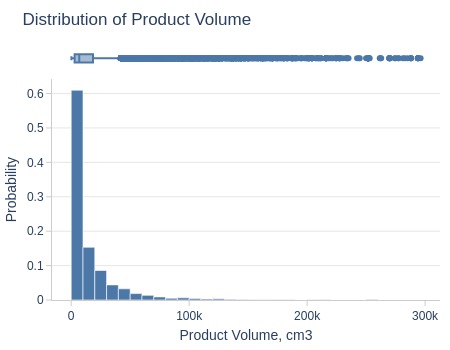
Key Observations:

• 75% of products have volume ≤19K cm3

• Top 5% ≥64K cm3

Weight to Volume Ratio

pb.configure(
    df = df_products
    , metric = 'weight_to_volume_ratio'
    , metric_label = 'Product Weight to Volume Ratio'
)

Top products.

pb.metric_top(id_column='product_id')

	weight_to_volume_ratio
product_id
2b752ed328ea866e4721ca4e236a416c	85.23
672ffb2231575afa70f7fee73fe400a1	65.91
fec8c282124bc6f504cbc6e9ec38450a	62.78
194dad3cf9aa121860ba80cca80331bb	48.15
30f902329cc4fd7dba514f7a5b629b2d	45.88
00ffe57f0110d73fd84d162252b2c784	45.45
29abbd57526dab494a667e62d361f6cf	40.06
b0c7a71c8620bd389e240f63a507dc50	37.78
c224f464aeeb2c6af33f0682a181efa7	35.80
0c22c51625fc11357a8356efa31fe89f	32.39

Let’s see at statistics and distribution of the metric.

pb.metric_info(
    upper_quantile=0.99
    , hist_mode='dual_hist_trim'    
)

Summary Statistics for "weight_to_volume_ratio" (Type: Float)

Summary			Percentiles			Detailed Stats			Value Counts
Total	32.95k (100%)		Max	85.23		Mean	0.20		0.08	1.85k (6%)
Missing	---		99%	1.22		Trimmed Mean (10%)	0.13		0.07	1.84k (6%)
Distinct	298 (<1%)		95%	0.52		Mode	0.08		0.05	1.74k (5%)
Non-Duplicate	113 (<1%)		75%	0.20		Range	85.23		0.06	1.70k (5%)
Duplicates	32.65k (99%)		50%	0.12		IQR	0.13		0.09	1.69k (5%)
Dup. Values	185 (<1%)		25%	0.07		Std	1.01		0.04	1.67k (5%)
Zeros	58 (<1%)		5%	0.03		MAD	0.09		0.10	1.52k (5%)
Negative	---		1%	0.01		Kurt	3.17k		0.11	1.38k (4%)
Memory Usage	<1 Mb		Min	0		Skew	50.31		0.17	1.38k (4%)

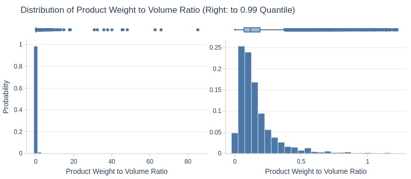
Key Observations:

• 75% of products have weight/volume ratio ≤0.2

• Top 5% ≥0.5

Other metrics

What fraction of products were not sold at all?

We have missing values in the number of sold units for products that were never sold.

products_no_sales_share = (df_products.total_units_sold.isna()).mean()

print(f'Share of Products with No Sales: {products_no_sales_share:.1%}')

Share of Products with No Sales: 2.5%