Customer Clustering#
All Customers#
Cluster Definition#
For clustering, we will use RFM metrics and the average number of unique products per order.
RFM metrics are well-suited for clustering. Adding the average number of unique products will help account for assortment demand diversity.
selected_metrics = [
    'avg_unique_products_cnt'
]
Create a dataframe with the selected metrics.
We will only consider customers who have made at least one successful purchase.
mask = df_customers.buys_cnt.notna()
cols_to_drop = ['recency_score', 'frequency_score', 'monetary_score', 'rfm_score', 'rfm_segment']
df_processed = (
    df_customers.loc[mask, ['customer_unique_id', *selected_metrics]]
    .merge(df_rfm, on='customer_unique_id', how='left')
    .drop(cols_to_drop, axis=1)
    .set_index('customer_unique_id')
)
Check for highly correlated features.
corr_matrix = df_processed.corr().abs()
upper_triangle = corr_matrix.where(np.triu(np.ones(corr_matrix.shape), k=1).astype(bool))
cols_to_drop = [column for column in upper_triangle.columns if any(upper_triangle[column] > 0.6)]
cols_to_drop
[]
No need to delete anything.
Look for missing values in the columns.
df_processed.isna().sum().nlargest(5)
avg_unique_products_cnt    0
recency                    0
frequency                  0
monetary                   0
dtype: int64
There are very few missing values, and they relate to customers who made only one purchase and have not yet received their item.
We will remove these rows before standardization.
scaler = StandardScaler()
df_processed = df_processed.dropna()
X_scaled = scaler.fit_transform(df_processed)
Determine the optimal number of clusters using the elbow method and silhouette analysis.
wcss = []
for i in range(1, 15):
    kmeans = KMeans(n_clusters=i, init='k-means++', random_state=42)
    kmeans.fit(X_scaled)
    wcss.append(kmeans.inertia_)

px.line(
    x=range(1, 15)
    , y=wcss
    , labels={'x': 'Number of clusters', 'y': 'WCSS'}
    , title='The Elbow Method'
    , width=600
    , height=400
)
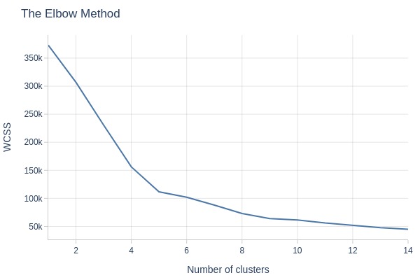
Key Observations:
The elbow method shows a clear break at 5 clusters. We’ll use 5 clusters.
optimal_clusters = 5
kmeans = KMeans(
    n_clusters=optimal_clusters
    , init='k-means++'
    , random_state=42)
cluster_labels = kmeans.fit_predict(X_scaled)
Examine quality
score = silhouette_score(X_scaled, cluster_labels)
print(f'Silhouette Score: {score:.3f}')
Silhouette Score: 0.492
Key Observations:
Silhouette score of 0.492 indicates good cluster separation.
Add cluster labels to the dataframe.
df_processed['cluster'] = cluster_labels + 1
Cluster Analysis#
Analyze the resulting clusters.
df_processed = df_processed.reset_index()
Distribution by Clustering Metrics
selected_metrics = [
    'avg_unique_products_cnt',
    'recency',
    'frequency',
    'monetary',
]
Provide more readable names for the metrics on the graphs.
metric_labels = {
    'avg_unique_products_cnt': 'Avg Unique Products',
    'recency': 'Recency',
    'frequency': 'Frequency',
    'monetary': 'Monetary',
}
cluster_label = {'cluster': 'Cluster'}
labels_for_polar={**cluster_label, **base_labels, **metric_labels}
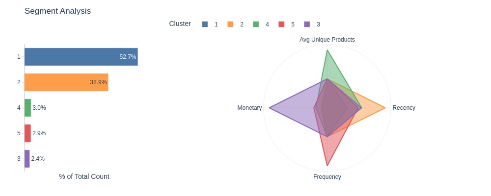
fig = df_processed.analysis.segment_polar(
    metrics=selected_metrics
    , dimension='cluster'
    , count_column='customer_unique_id'
    , labels=labels_for_polar
)
pb.to_slide(fig, 'cluster all')
fig.show()
df_processed.analysis.segment_table(
    metrics=selected_metrics
    , dimension='cluster'
    , count_column='customer_unique_id'
)
fig.show()
| cluster | 3 | 4 | 5 | 2 | 1 |
|---|---|---|---|---|---|
| % of Total Count | 2.42% | 3.03% | 2.95% | 38.95% | 52.66% |
| avg_unique_products_cnt | 1.00 | 2.00 | 1.00 | 1.00 | 1.00 |
| recency | 218.50 | 221.00 | 197.50 | 372.00 | 128.00 |
| frequency | 1.00 | 1.00 | 2.00 | 1.00 | 1.00 |
| monetary | 966.53 | 187.81 | 223.66 | 99.43 | 101.75 |
Key Observations:
Most customers fall in Cluster 1 (53%) and Cluster 2 (39%).
Cluster 1: No standout metrics
Cluster 2: Highest Recency
Cluster 3: Highest Monetary, Cluster 4: Highest Avg Unique Products, Cluster 5: Highest Frequency
Number of Customers by Clusters in Different Segments
Add dimensions to the dataframe with clusters.
df_processed = (
    df_processed.merge(df_customers[['customer_unique_id', *customers_dim]], on='customer_unique_id', how='left')
)
df_processed.viz.update_plotly_settings(
    labels={**base_labels, 'cluster': 'Cluster'}
)
pb.configure(
    df = df_processed
    , metric = 'customer_unique_id'
    , metric_label = 'Share of Customers'
    , agg_func = 'nunique'
    , norm_by='all'
    , axis_sort_order='descending'
    , text_auto='.1%'
    , plotly_kwargs= {'category_orders': {'cluster': list(range(1, 6))}}
)
By Activity Segment
pb.cat_compare(
    cat1='cluster'
    , cat2 = 'activity_segment'
    , visible_graphs = [2, 3]
)
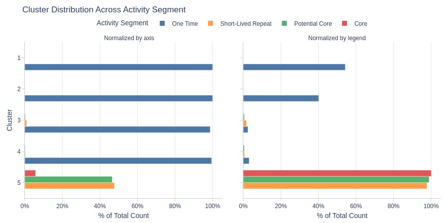
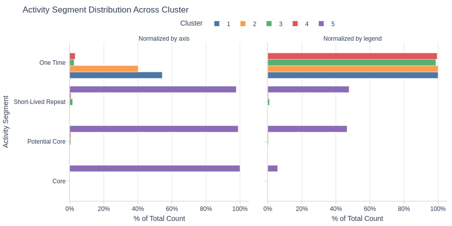
Key Observations:
Clusters 1-4 are dominated by one-time purchasers.
Cluster 5 dominates all active segments except one-time purchases.
One-time purchase rates are similar across all clusters except Cluster 5.
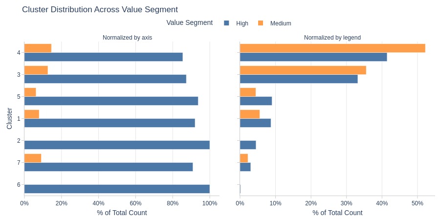
By Purchase Amount Segment
pb.cat_compare(
    cat1='cluster'
    , cat2 = 'value_segment'
    , visible_graphs = [2, 3]
)
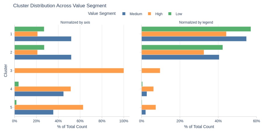
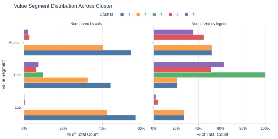
Key Observations:
Clusters 1-2: Mostly medium payment tier
Cluster 3: Entirely high-value segment
Clusters 1-2 are less common in high-value segment
Clusters 1-2 dominate within each value segment
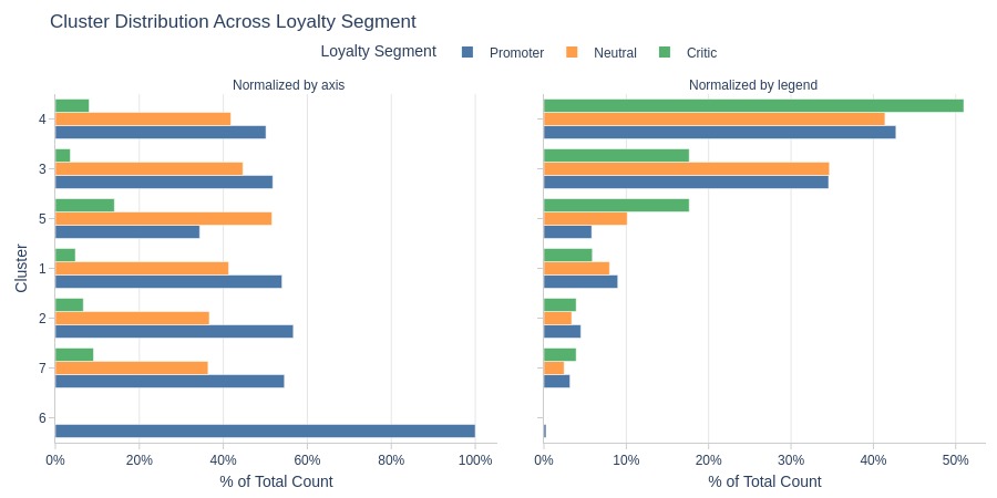
By Loyalty Segment
pb.cat_compare(
    cat1='cluster'
    , cat2 = 'loyalty_segment'
    , visible_graphs = [2, 3]
)
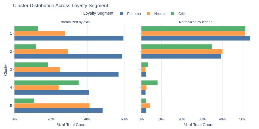
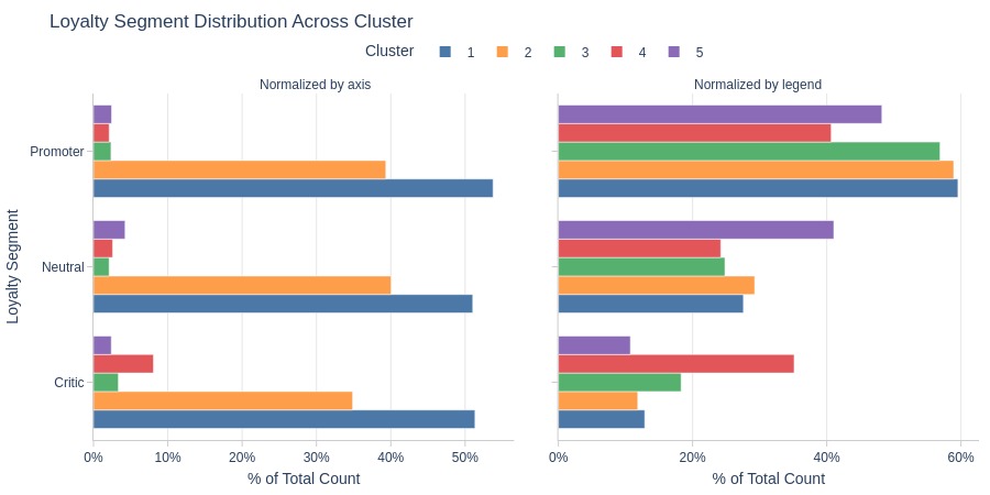
Key Observations:
Cluster 4 has notably more critics
Clusters 1-2 dominate across loyalty segments
Fewer promoters in Cluster 4
More neutrals in Cluster 5
More critics in Cluster 4
By Risk Segment
pb.cat_compare(
    cat1='cluster'
    , cat2 = 'risk_segment'
    , visible_graphs = [2, 3]
)
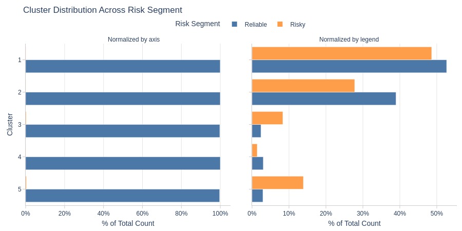
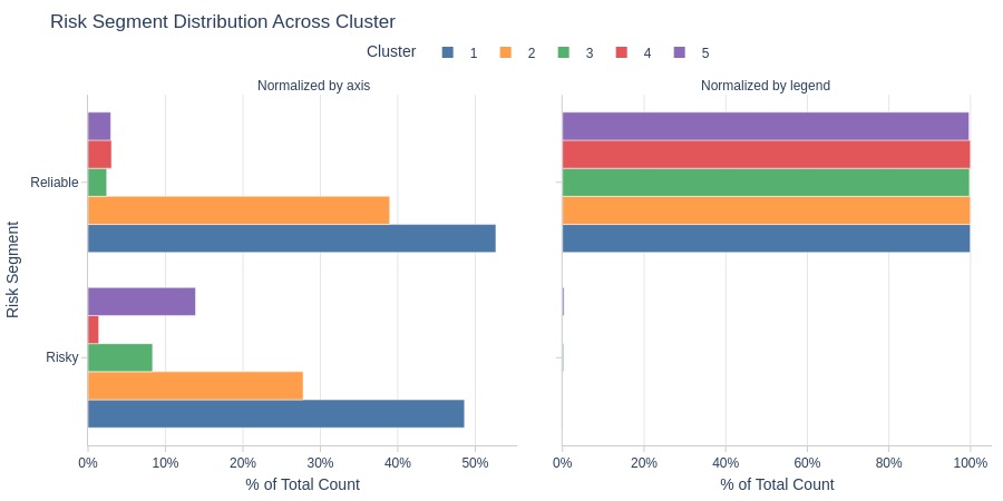
Key Observations:
Clusters 4-5 are more common among risky customers (with order cancellations)
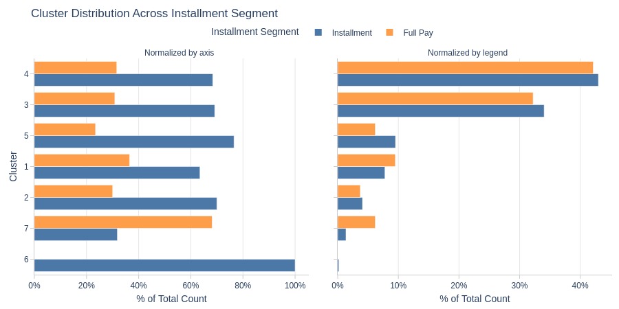
By Installment Segment
pb.cat_compare(
    cat1='cluster'
    , cat2 = 'installment_segment'
    , visible_graphs = [2, 3]
)
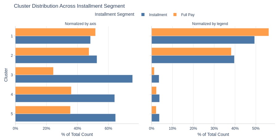
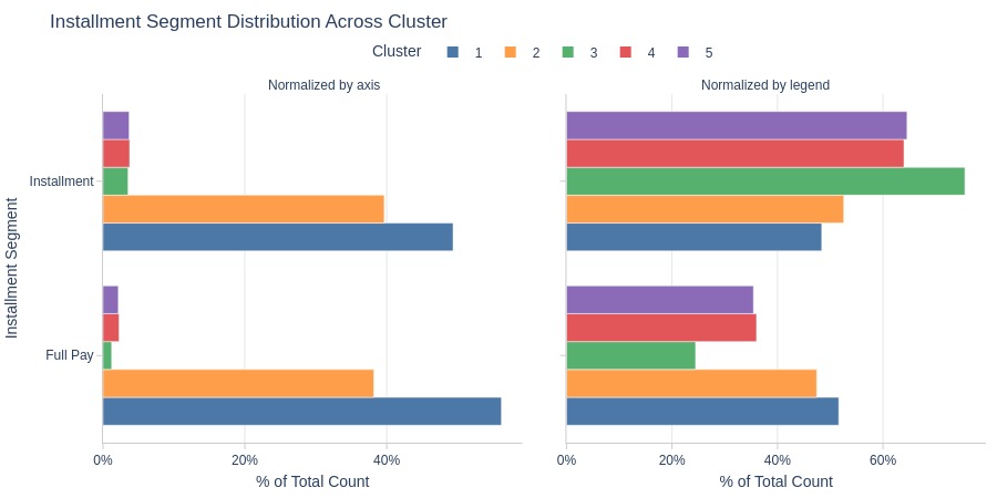
Key Observations:
Installments don’t dominate Clusters 1-2
Installments clearly dominate Clusters 3-5
Highest installment rate in Cluster 3
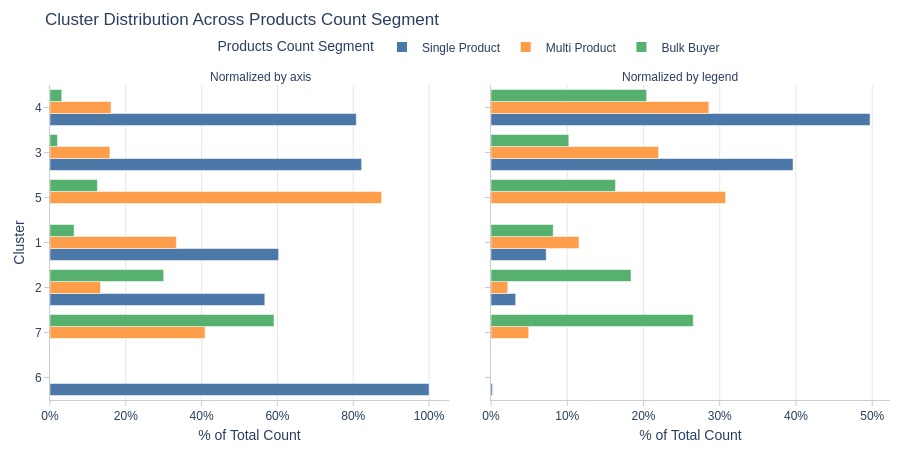
By Average Number of Products per Order Segment
pb.cat_compare(
    cat1='cluster'
    , cat2 = 'products_cnt_segment'
    , visible_graphs = [2, 3]
)
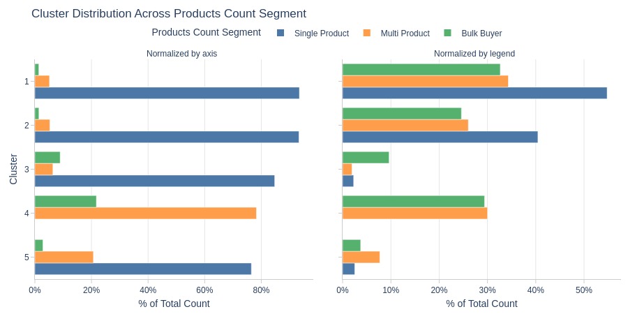

Key Observations:
Cluster 4 consists entirely of customers averaging >1 product per order
By Average Order Weight Segment
pb.cat_compare(
    cat1='cluster'
    , cat2 = 'weight_segment'
    , visible_graphs = [2, 3]
)
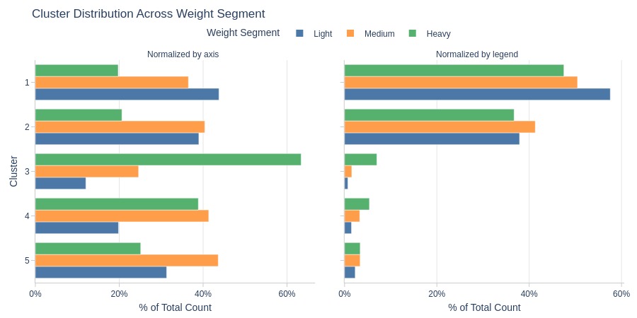
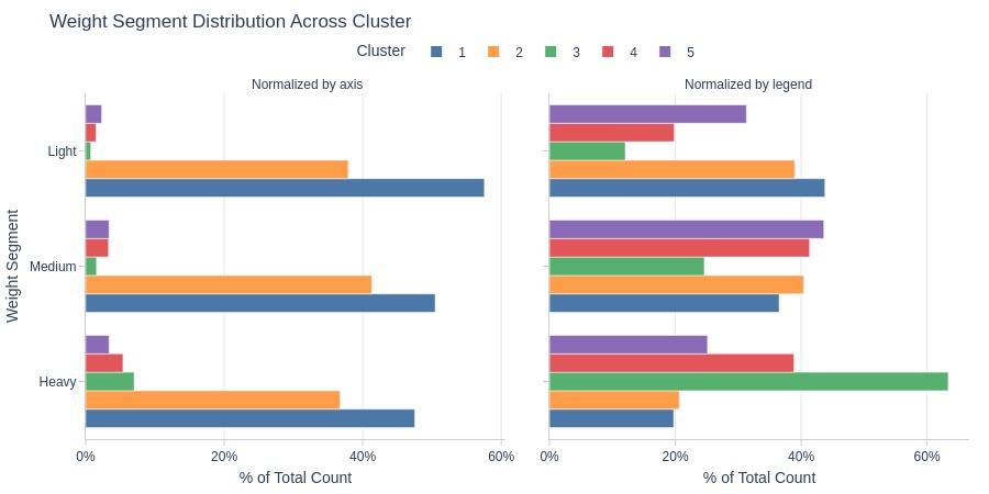
Key Observations:
Cluster 3 has more heavy-weight orders
Cluster 1 dominates light-weight orders
By Top Payment Types
pb.cat_compare(
    cat1='cluster'
    , cat2 = 'customer_payment_types'
    , trim_top_n_cat2=5
    , visible_graphs = [2, 3]
)
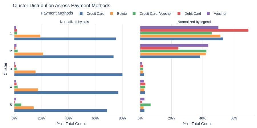
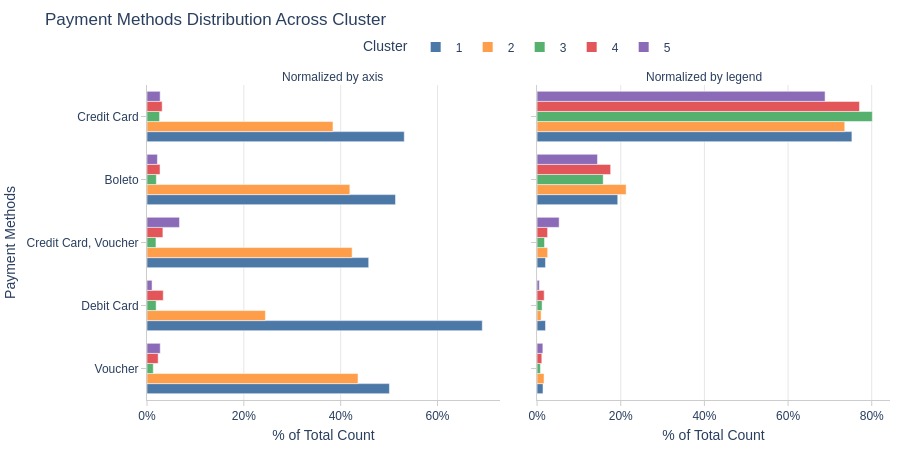
Key Observations:
Cluster 1 has more debit card users
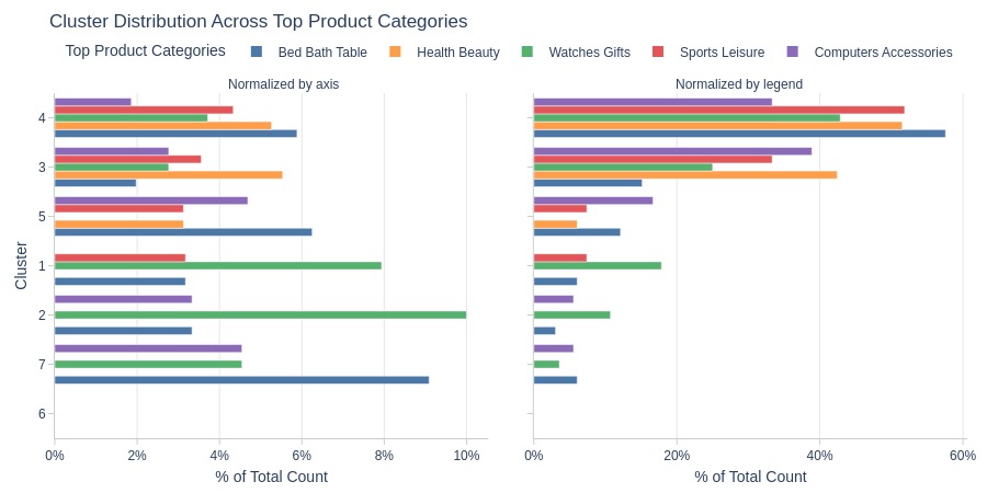
By Top Product Categories
pb.cat_compare(
    cat1='cluster'
    , cat2 = 'customer_top_product_categories'
    , trim_top_n_cat2=5
    , visible_graphs = [2, 3]
)
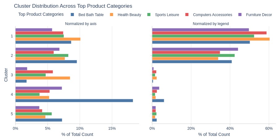
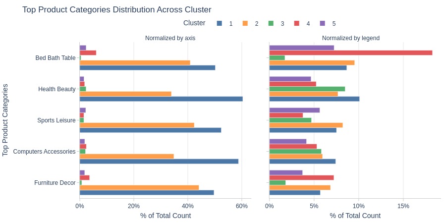
Key Observations:
Cluster 4 dominates Bed Bath Table category
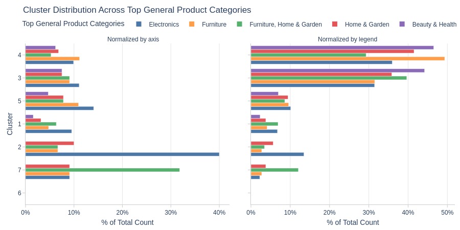
By Top Generalized Product Categories
pb.cat_compare(
    cat1='cluster'
    , cat2 = 'customer_top_general_product_categories'
    , trim_top_n_cat2=5
    , visible_graphs = [2, 3]
)
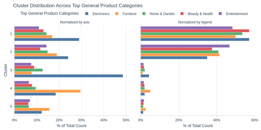
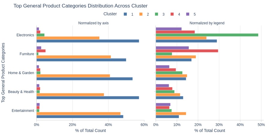
Key Observations:
Cluster 3: Dominated by electronics
Cluster 4: Dominated by furniture
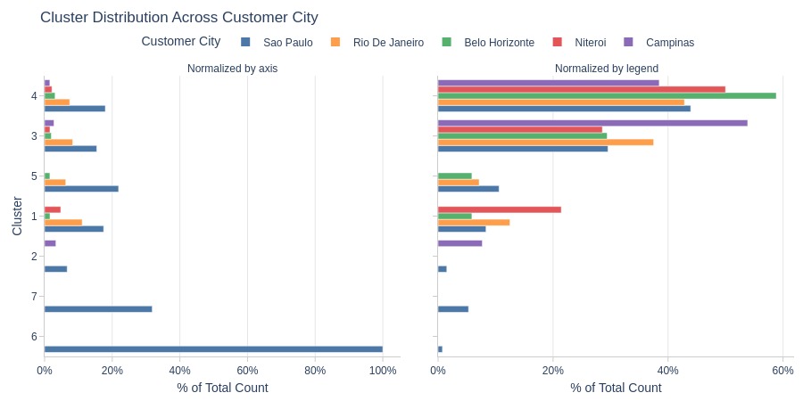
By Customer State
pb.cat_compare(
    cat1='cluster'
    , cat2 = 'customer_city'
    , trim_top_n_cat2=5
    , visible_graphs = [2, 3]
)
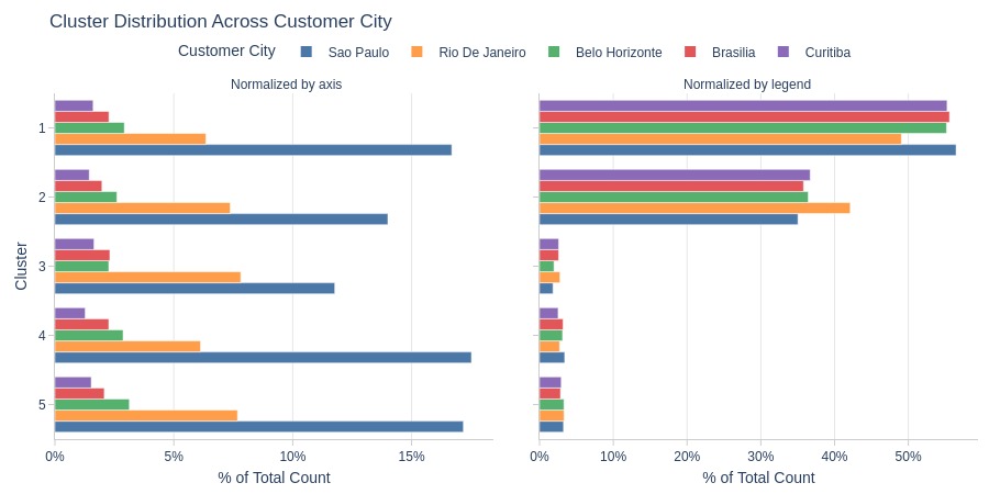
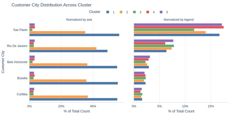
Key Observations:
Cluster 2 is more common in Rio de Janeiro
Cluster 1 is less common in Rio de Janeiro
Customers with Multiple Purchases#
Cluster Definition#
We will conduct a separate clustering of customers who have made more than one successful purchase.
We will use the same metrics as in the clustering of all customers.
selected_metrics = [
    'avg_unique_products_cnt'
]
mask = df_customers.buys_cnt >= 2
cols_to_drop = ['recency_score', 'frequency_score', 'monetary_score', 'rfm_score', 'rfm_segment']
df_processed = (
    df_customers.loc[mask, ['customer_unique_id', *selected_metrics]]
    .merge(df_rfm[lambda x: x.rfm_segment=='Champions'], on='customer_unique_id', how='inner')
    .drop(cols_to_drop, axis=1)
    .set_index('customer_unique_id')
)
Check for missing values.
df_processed.isna().sum().nlargest(5)
avg_unique_products_cnt    0
recency                    0
frequency                  0
monetary                   0
dtype: int64
There are no missing values.
scaler = StandardScaler()
df_processed = df_processed.dropna()
X_scaled = scaler.fit_transform(df_processed)
Determine the optimal number of clusters using the silhouette method.
silhouette_scores = []
for n_clusters in range(2, 15):
    kmeans = KMeans(n_clusters=n_clusters, random_state=42)
    cluster_labels = kmeans.fit_predict(X_scaled)
    silhouette_avg = silhouette_score(X_scaled, cluster_labels)
    silhouette_scores.append(silhouette_avg)
px.line(
    x=range(2, 15)
    , y=silhouette_scores
    , labels={'x': 'Number of clusters', 'y': 'Silhouette Score'}
    , title='Silhouette Score Method'
    , width=600
    , height=400
)
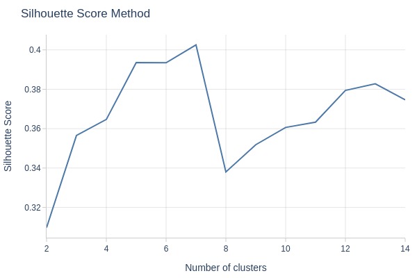
Key Observations:
Global peak at 7 clusters
Sharp drop after k=7 suggests overfitting
Examine the dendrogram of hierarchical clustering.
linked = linkage(X_scaled, method='ward')
fig = ff.create_dendrogram(
    linked
    , orientation='bottom'
)
fig.update_layout(
    title='Dendrogram of hierarchical clustering',
    xaxis_title='Observations',
    yaxis_title='Distance',
    width=800,
    height=500,
    margin=dict(l=50, r=50, b=50, t=50),
    yaxis_mirror=False,
)
fig.update_xaxes(showticklabels=False, ticks='', mirror=False)
fig.show(config=dict(displayModeBar=False), renderer="png")
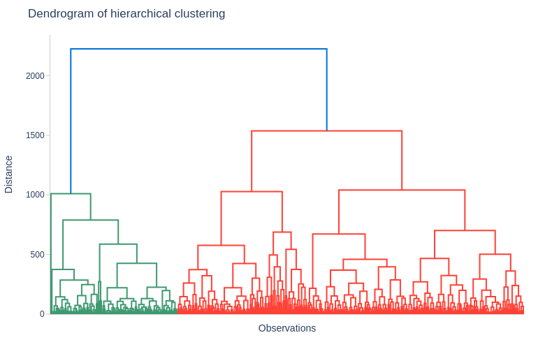
Key Observations:
Optimal cut at 6-7 clusters (where branches lengthen)
We’ll choose 7 clusters
optimal_clusters = 7
model = AgglomerativeClustering(n_clusters=optimal_clusters)
cluster_labels = model.fit_predict(X_scaled)
Evaluate quality.
score = silhouette_score(X_scaled, cluster_labels)
print(f'Silhouette Score: {score:.3f}')
Silhouette Score: 0.410
Key Observations:
Silhouette score of 0.41 indicates good clustering
Clusters remain distinguishable despite score <0.5
Add cluster labels to the dataframe.
df_processed['cluster'] = cluster_labels + 1
Cluster Analysis#
Analyze the resulting clusters.
df_processed = df_processed.reset_index()
Distribution by Clustering Metrics
selected_metrics = [
    'avg_unique_products_cnt',
    'recency',
    'frequency',
    'monetary',
]
Provide more readable names for the metrics on the graphs.
metric_labels = {
    'avg_unique_products_cnt': 'Avg Unique Products',
    'recency': 'Recency',
    'frequency': 'Frequency',
    'monetary': 'Monetary',
}
cluster_label = {'cluster': 'Cluster'}
labels_for_polar={**cluster_label, **base_labels, **metric_labels}
fig = df_processed.analysis.segment_polar(
    metrics=selected_metrics
    , dimension='cluster'
    , count_column='customer_unique_id'
    , labels=labels_for_polar
)
pb.to_slide(fig, 'cluster repeat')
fig.show()
df_processed.analysis.segment_table(
    metrics=selected_metrics
    , dimension='cluster'
    , count_column='customer_unique_id'
)
fig.show()
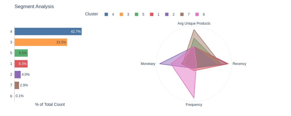
| cluster | 2 | 6 | 7 | 1 | 5 | 4 | 3 |
|---|---|---|---|---|---|---|---|
| % of Total Count | 3.97% | 0.13% | 2.91% | 8.33% | 8.47% | 42.72% | 33.47% |
| avg_unique_products_cnt | 1.00 | 1.00 | 2.00 | 1.00 | 1.50 | 1.00 | 1.00 |
| recency | 67.00 | 8.00 | 83.50 | 107.00 | 80.00 | 103.00 | 28.00 |
| frequency | 2.00 | 15.00 | 2.00 | 3.00 | 2.00 | 2.00 | 2.00 |
| monetary | 1308.12 | 879.27 | 432.62 | 480.52 | 311.05 | 266.76 | 291.46 |
Key Observations:
Most customers in Cluster 4 (43%) and Cluster 3 (34%)
Cluster 1: No standout metrics
Cluster 2: Highest Monetary
Cluster 6: High Frequency and Monetary
Cluster 7: High avg unique products
Number of Customers by Clusters in Different Segments
Add dimensions to the dataframe with clusters.
df_processed = (
    df_processed.merge(df_customers[['customer_unique_id', *customers_dim]], on='customer_unique_id', how='left')
)
df_processed.viz.update_plotly_settings(
    labels={**base_labels, 'cluster': 'Cluster'}
)
pb.configure(
    df = df_processed
    , metric = 'customer_unique_id'
    , metric_label = 'Share of Customers'
    , agg_func = 'nunique'
    , norm_by='all'
    , axis_sort_order='descending'
    , text_auto='.1%'
)
By Activity Segment
pb.cat_compare(
    cat1='cluster'
    , cat2 = 'activity_segment'
    , visible_graphs = [2, 3]
)
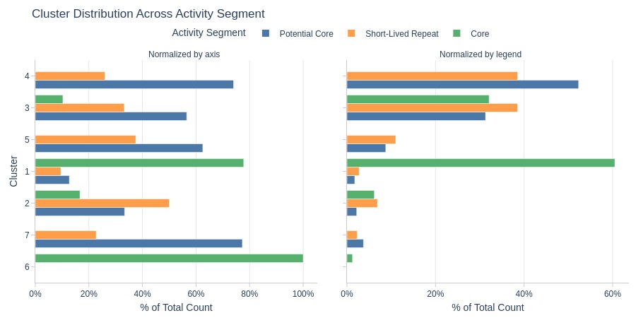
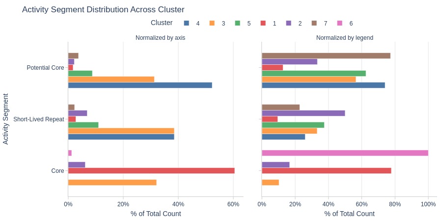
Key Observations:
Cluster 6: Entirely core audience
Core also dominates Cluster 1
Cluster 4 dominates potential core segment
By Purchase Amount Segment
pb.cat_compare(
    cat1='cluster'
    , cat2 = 'value_segment'
    , visible_graphs = [2, 3]
)
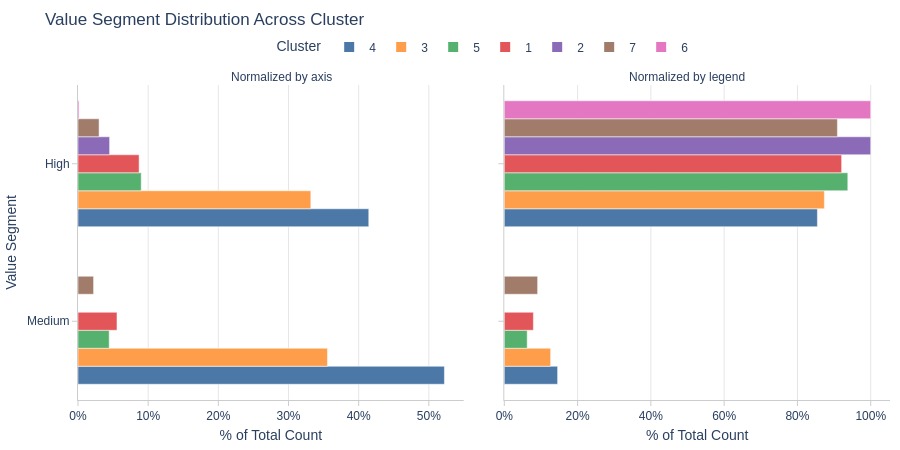
Key Observations:
Clusters 2 and 6: Entirely high-value segment
Cluster 4 dominates medium-value segment
By Loyalty Segment
pb.cat_compare(
    cat1='cluster'
    , cat2 = 'loyalty_segment'
    , visible_graphs = [2, 3]
)
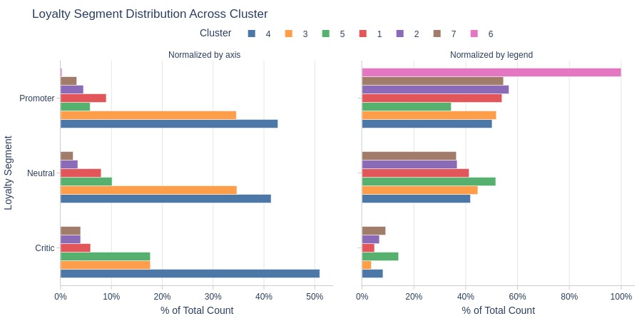
Key Observations:
Cluster 6: Entirely promoters
Cluster 4 dominates critics
Clusters 4-5 more common among critics
By Installment Segment
pb.cat_compare(
    cat1='cluster'
    , cat2 = 'installment_segment'
    , visible_graphs = [2, 3]
)
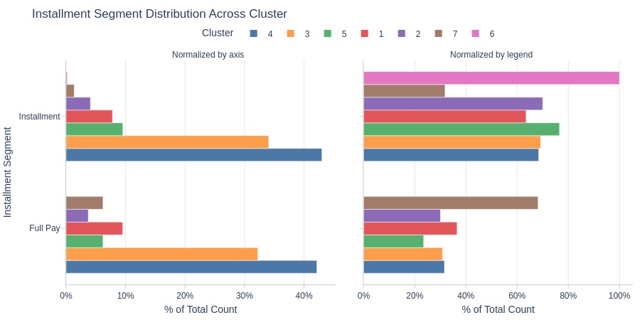
Key Observations:
Cluster 6: Entirely installment users
Cluster 7 has more full-payment users
By Average Number of Products per Order Segment
pb.cat_compare(
    cat1='cluster'
    , cat2 = 'products_cnt_segment'
    , visible_graphs = [2, 3]
)
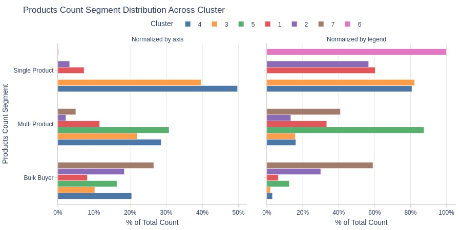
Key Observations:
Cluster 6: Entirely single-product orders
Cluster 7: No single-product orders
Clusters 3-4 dominate single-product orders
Clusters 2 and 7 dominate bulk orders (>2 products)
Cluster 5 has more multi-product orders
By Average Order Weight Segment
pb.cat_compare(
    cat1='cluster'
    , cat2 = 'weight_segment'
    , visible_graphs = [2, 3]
)
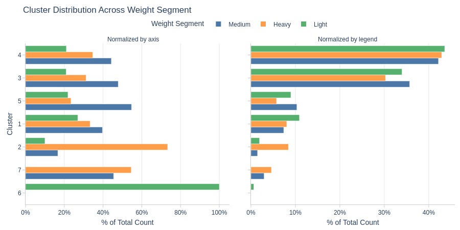
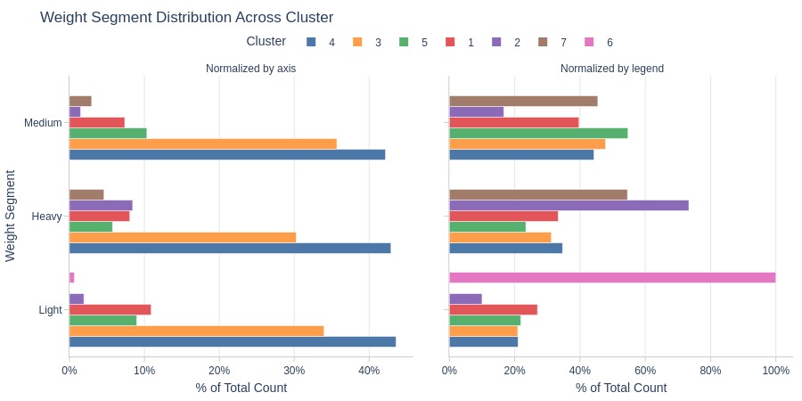
Key Observations:
Cluster 6: Entirely light-weight orders
Cluster 2: Heavy-weight orders dominate
By Top Payment Types
pb.cat_compare(
    cat1='cluster'
    , cat2 = 'customer_payment_types'
    , trim_top_n_cat2=5
    , visible_graphs = [2, 3]
)
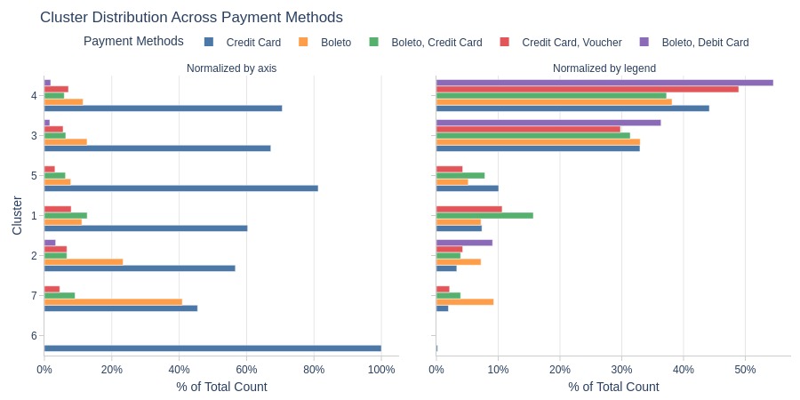
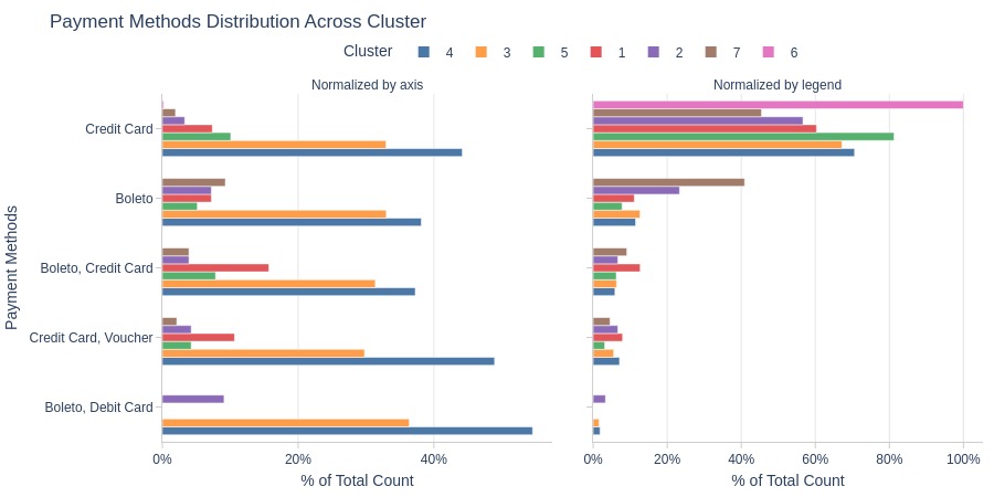
Key Observations:
Cluster 6: Entirely credit card users
Cluster 7 has more boleto users
By Top Product Categories
pb.cat_compare(
    cat1='cluster'
    , cat2 = 'customer_top_product_categories'
    , trim_top_n_cat2=5
    , visible_graphs = [2, 3]
)
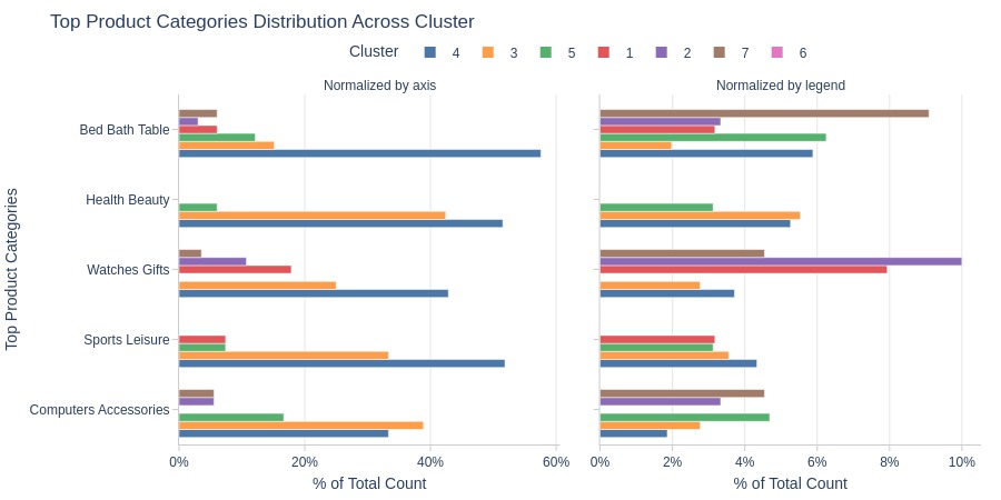
Key Observations:
Clusters 1-2 dominate Watches Gifts category
Cluster 7 dominates Bed Bath Table
By Top Generalized Product Categories
pb.cat_compare(
    cat1='cluster'
    , cat2 = 'customer_top_general_product_categories'
    , trim_top_n_cat2=5
    , visible_graphs = [2, 3]
)
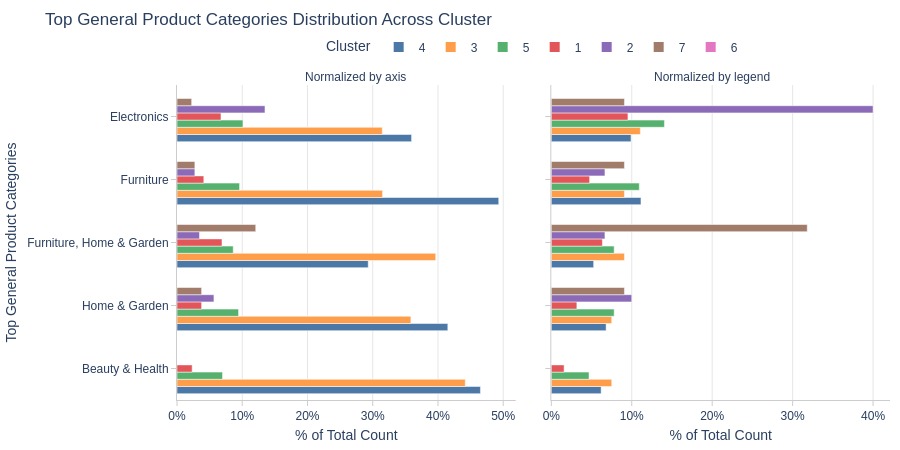
Key Observations:
Cluster 2 strongly dominates electronics
Cluster 7 dominates furniture and home/garden
By Customer State
pb.cat_compare(
    cat1='cluster'
    , cat2 = 'customer_city'
    , trim_top_n_cat2=5
    , visible_graphs = [2, 3]
)
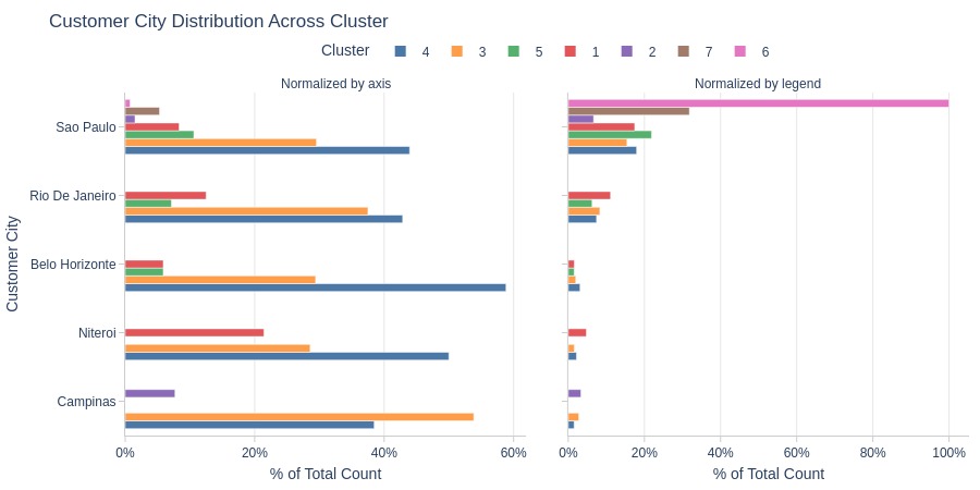
Key Observations:
Cluster 6: Entirely São Paulo customers (top 5 cities)
Cluster 1 more common in Niterói
Cluster 3 more common in Campinas