RFM Analysis

rfm_res = df_sales.analysis.rfm(
    user_id_col='customer_unique_id'
    , order_id_col='order_id'
    , date_col='order_purchase_dt'
    , revenue_col='total_payment'
    , upper_quantile=0.99
    , return_rfm=True
)

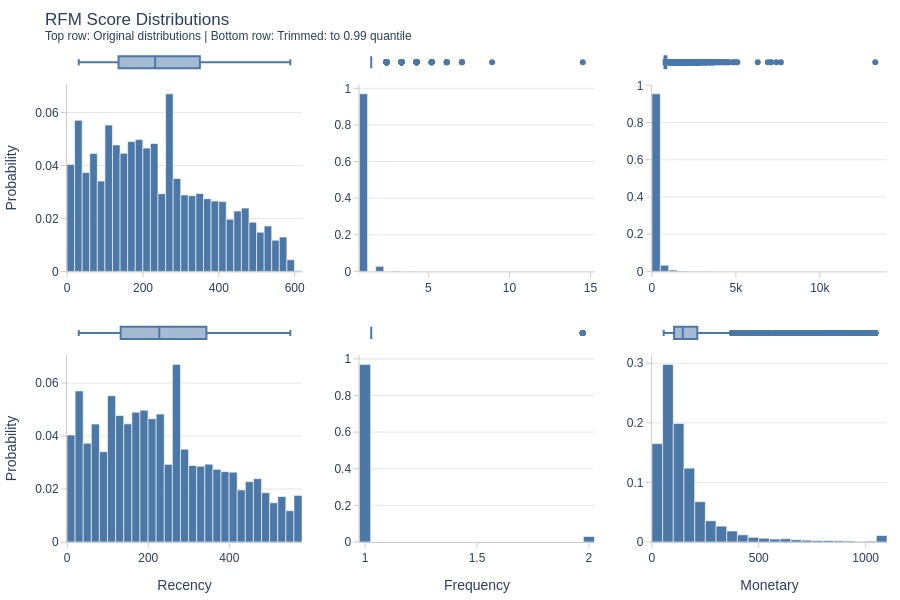
Let’s examine the distributions of Recency, Frequency, and Monetary.

rfm_res['hist']

Let’s look at the RFM heatmap where color represents Monetary.

fig = rfm_res['heat']
pb.to_slide(fig)
fig.show()

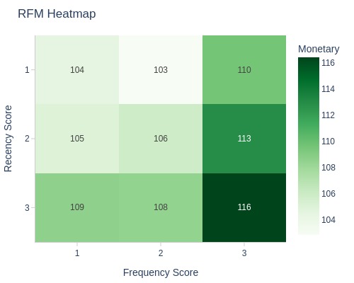
Key Observations:

• The FR segment 33 generates the highest payments - frequent recent buyers.

Let’s examine the distribution of customers by RFM pairwise combinations.

fig = rfm_res['heat_pairs']
pb.to_slide(fig)
fig.show()

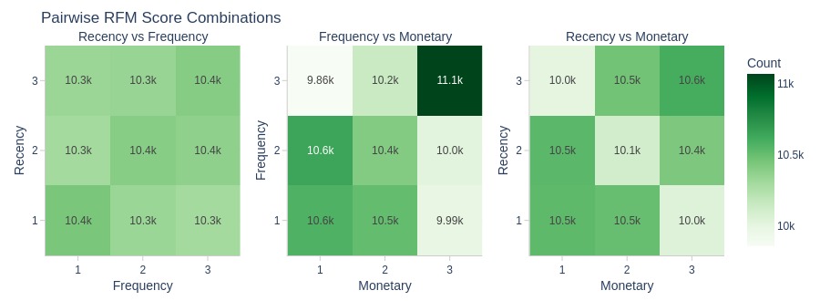
Key Observations:

• The FM segment 33 clearly stands out in terms of customer count - frequent high-value buyers.

Let’s examine slices of the FM pair by R.

fig = rfm_res['heat_sliced']
pb.to_slide(fig)
fig.show()

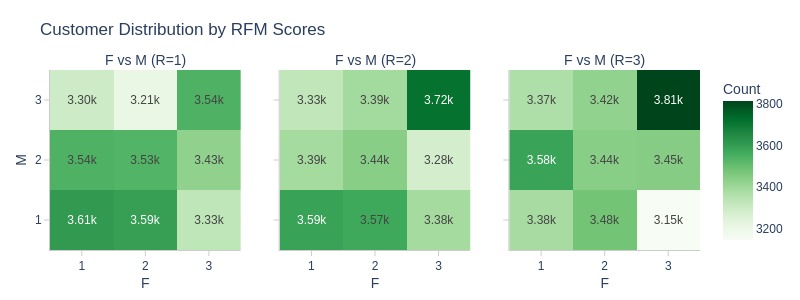
Key Observations:

• The FM33 segment contains the most R=3 customers - frequent recent high-value buyers.

Let’s look at the distribution by segments.

fig_tree = rfm_res['seg_tree']
fig_bar = rfm_res['seg_bar']
pb.to_slide(fig_tree, '_treemap')
pb.to_slide(fig_bar, '_bar')
fig_tree.show()
fig_bar.show()

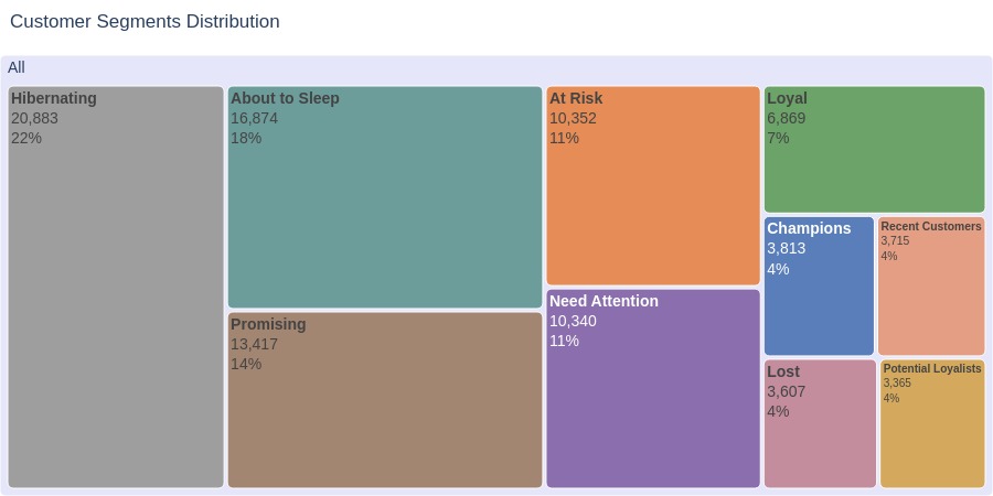
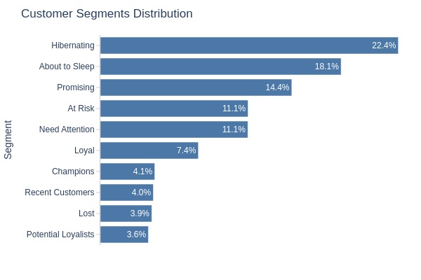
Key Observations:

• Largest segments: Hibernating (22%), About to Sleep (18%), Promising (14%) - mostly inactive customers.

• Champions: 4%, Loyal: 7%, Lost: 4%.

Save the RFM dataframe for clustering.

df_rfm = rfm_res['df_rfm']
del rfm_res