Delivery Analysis

Delivery Cost

pb.configure(
    df = df_sales
    , time_column = 'order_purchase_dt'
    , metric = 'total_freight_value'
    , metric_label = 'Average Freight Value per Order, R$'
    , metric_label_for_distribution = 'Freight Value per Order, R$'
    , agg_func = 'mean'
    , axis_sort_order='descending'
    , text_auto='.3s'
)

print(f'Average Freight Value per Order: {df_sales.total_freight_value.mean():.2f} R$')

Average Freight Value per Order: 22.78 R$

Top Orders.

pb.metric_top()

	total_freight_value
order_id
cf4659487be50c0c317cff3564c4a840	1,794.96
2455cbeb73fd04b170ca2504662f95ce	1,002.29
cfed507ac357129f750f05a0d7d71b15	711.33
71dab1155600756af6de79de92e712e3	626.64
17784b9fbb37fb0bdc230d8ed6f6b355	502.98
725cf8e9c24e679a8a5a32cb92c9ce1e	497.42
5bd06bab48e0423fc35d1c236d48a6bb	497.08
be382a9e1ed25128148b97d6bfdb21af	479.28
c52c7fbe316b5b9d549e8a25206b8a1f	458.73
62073ec6b54b8e6322037fc0f3591ad3	456.47

Let’s see at statistics and distribution of the metric.

pb.metric_info(
    upper_quantile=0.95
    , hist_mode='dual_hist_trim'    
)

Summary Statistics for "total_freight_value" (Type: Float)

Summary			Percentiles			Detailed Stats			Value Counts
Total	96.35k (100%)		Max	1.79k		Mean	22.78		15.10	2.90k (3%)
Missing	---		99%	104.24		Trimmed Mean (10%)	19.03		7.78	1.80k (2%)
Distinct	7.87k (8%)		95%	54.74		Mode	15.10		14.10	1.49k (2%)
Non-Duplicate	2.80k (3%)		75%	24.01		Range	1.79k		11.85	1.42k (1%)
Duplicates	88.48k (92%)		50%	17.17		IQR	10.16		18.23	1.20k (1%)
Dup. Values	5.07k (5%)		25%	13.85		Std	21.57		7.39	1.13k (1%)
Zeros	336 (<1%)		5%	7.87		MAD	6.49		15.23	811 (<1%)
Negative	---		1%	7.39		Kurt	586.22		16.11	780 (<1%)
Memory Usage	1		Min	0		Skew	12.28		8.72	738 (<1%)

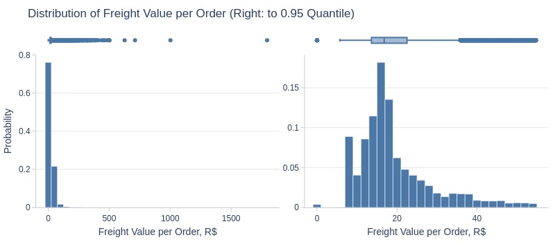
Key Observations:

• 75% of orders have shipping costs ≤24 R$

• Top 5% have shipping costs ≥54.7 R$

• Several extreme outliers exist with very high shipping costs

pb.metric_top(freq='D')

	total_freight_value
order_purchase_dt
2017-06-20	33.28
2018-07-02	32.34
2017-06-21	31.19
2017-04-18	30.24
2018-07-15	29.37
2018-07-13	29.25
2018-07-01	29.10
2017-06-25	28.90
2018-07-11	28.78
2017-11-04	28.69

Let’s look by different dimensions.

By Whether the Order is Delayed or Not

pb.histogram(
    color='is_delayed'
    , upper_quantile=0.95
    , mode='dual_box_trim'
    , show_box=True
    , show_hist=False
    , show_kde=True
    , nbins=30
).show()
pb.bar_groupby(
    y='is_delayed'
    , show_count=True
).show()

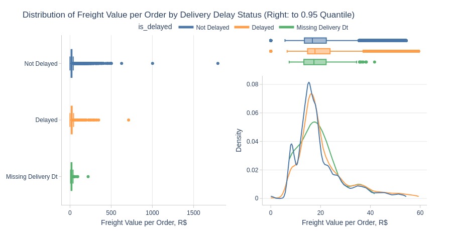
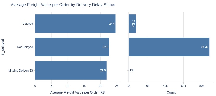
Key Observations:

• Delayed orders have higher shipping costs than non-delayed

By Order Weight Category

pb.histogram(
    color='order_total_weight_cat'
    , upper_quantile=0.95
    , mode='dual_box_trim'
    , show_box=True
    , show_hist=True
    , show_kde=False
    , nbins=30
).show()
pb.bar_groupby(
    y='order_total_weight_cat'
).show()

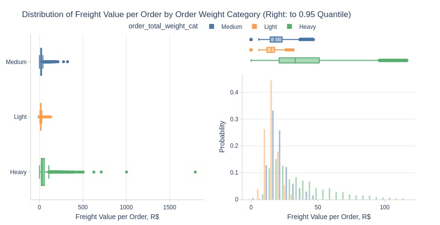
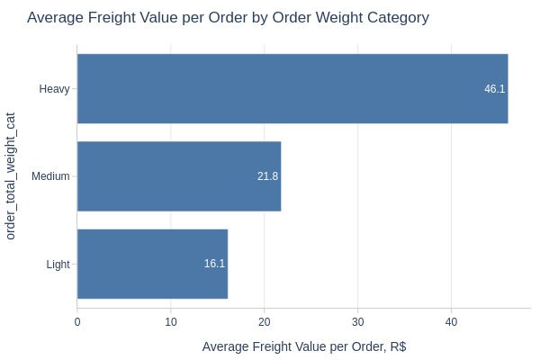
Key Observations:

• Heavier orders have higher shipping costs (expected pattern)

By Presence of Installment Payments

pb.histogram(
    color='order_has_installment'
    , upper_quantile=0.95
    , mode='dual_box_trim'
    , show_box=True
    , show_hist=True
    , show_kde=False
    , nbins=30
).show()
pb.bar_groupby(
    y='order_has_installment'
    , show_count=True
    , to_slide=True
).show()

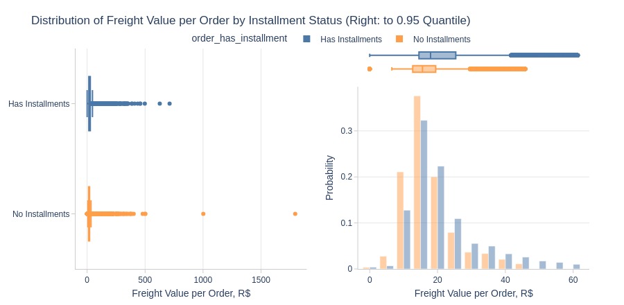
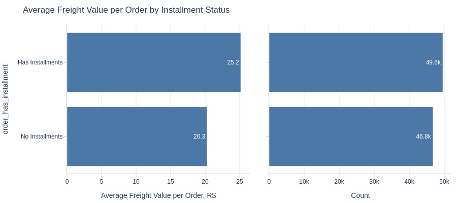
Key Observations:

• Installment orders have higher shipping costs

By Top Customer States

pb.box(
    y='customer_state'
    , upper_quantile=0.95
    , show_dual=True
).show()
fig = pb.bar_groupby(
    y='customer_state'
    , show_count=True
).update_layout(xaxis2_title_text='Number of Sales')
pb.to_slide(fig)
fig.show()

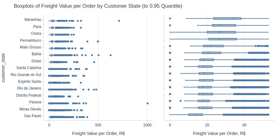
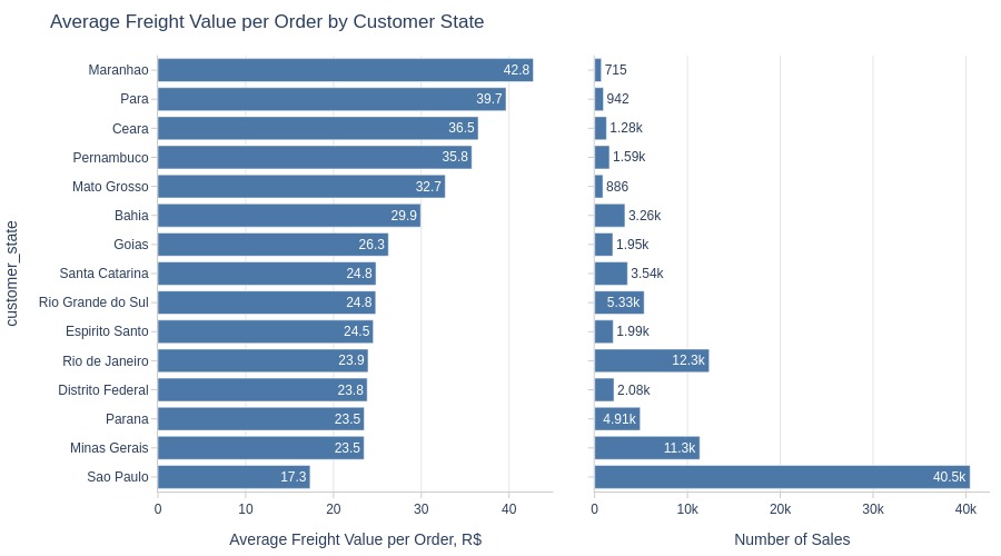
Key Observations:

• Among top states by sales volume:

  • São Paulo has lowest average shipping costs

  • Maranhão has highest

By Top Customer Cities

pb.box(
    y='customer_city'
    , upper_quantile=0.95
    , show_dual=True
).show()
pb.bar_groupby(
    y='customer_city'
    , show_count=True
).update_layout(xaxis2_title_text='Number of Sales')

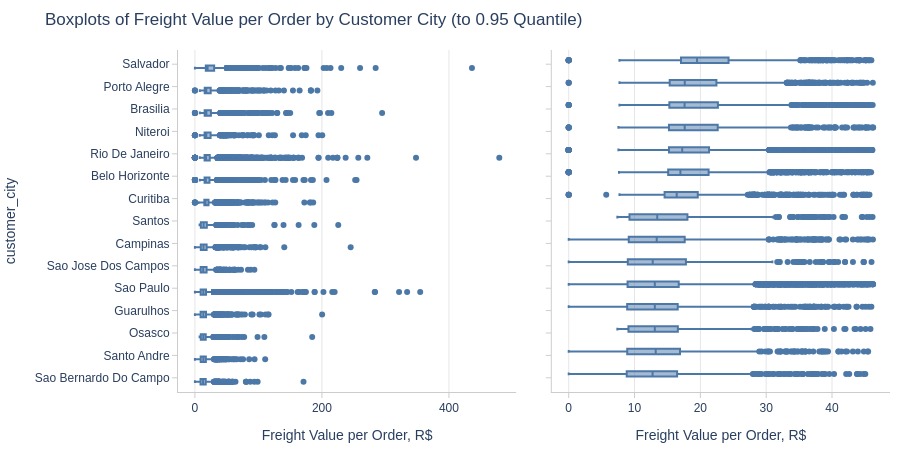
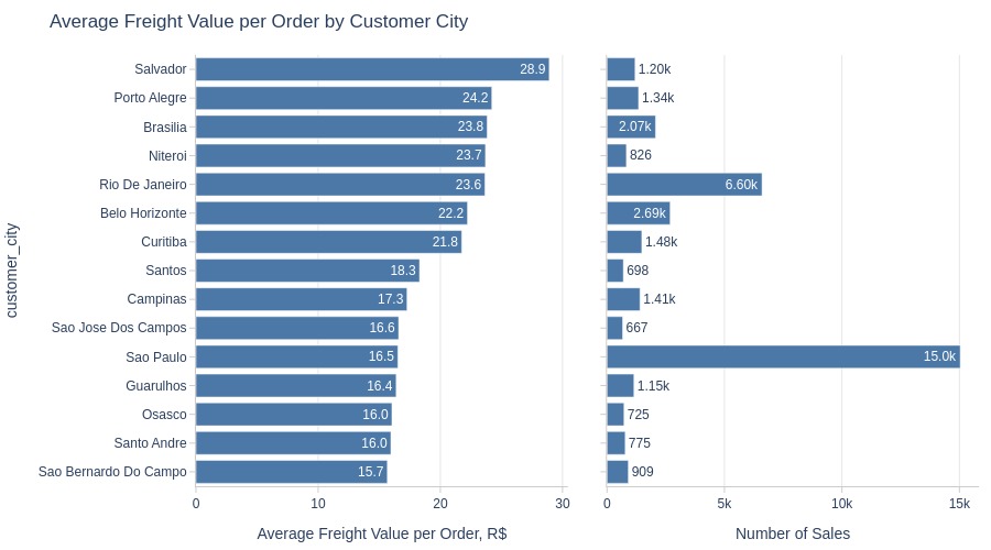
Key Observations:

• Among top cities by sales volume, highest average shipping costs in:

  1. Salvador

  2. Porto Alegre

  3. Brasília

By Review Score

pb.histogram(
    color='order_avg_reviews_score'
    , upper_quantile=0.95
    , mode='dual_box_trim'
    , show_box=True
    , show_hist=False
    , show_kde=True
    , nbins=30
).show()
fig = pb.bar_groupby(
    y='order_avg_reviews_score'
    , show_count=True
).update_layout(xaxis2_title_text='Number of Sales')
pb.to_slide(fig)
fig.show()

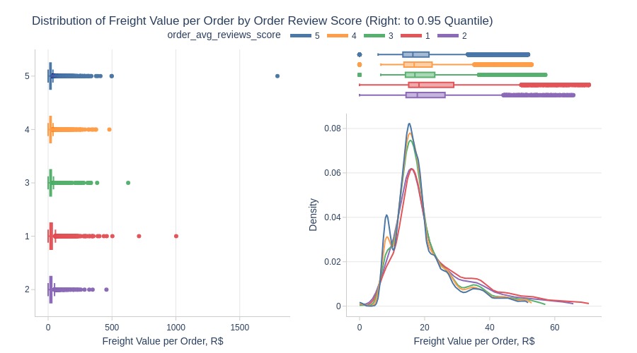
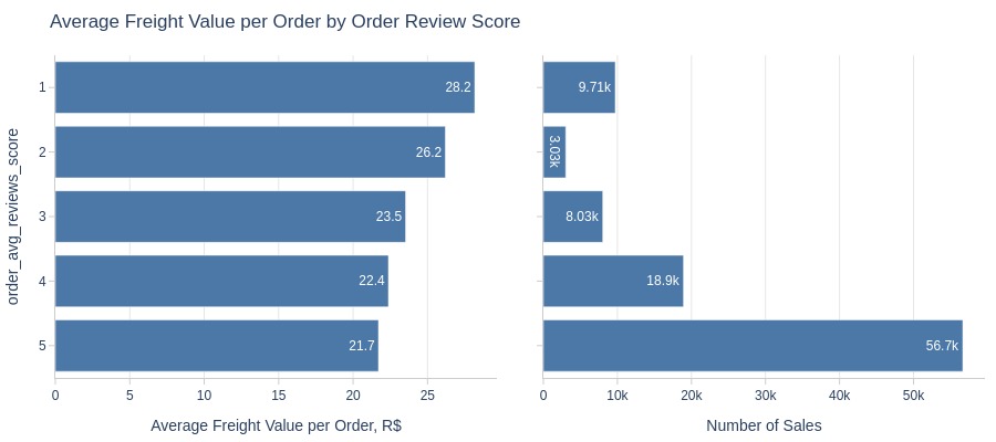
Key Observations:

• Higher shipping costs correlate with lower order ratings

Distance Between Customer and Seller

pb.configure(
    df = df_sales
    , time_column = 'order_purchase_dt'
    , metric = 'avg_distance_km'
    , metric_label = 'Average Distance, km'
    , metric_label_for_distribution = 'Average Distance, km'
    , agg_func = 'mean'
    , axis_sort_order='descending'
    , text_auto='.1f'
)

print(f'Average Distance: {df_sales.avg_distance_km.mean():.2f} km')

Average Distance: 600.55 km

Let’s see at statistics and distribution of the metric.

pb.metric_info(
    upper_quantile=0.95
    , hist_mode='dual_hist_trim'    
)

Summary Statistics for "avg_distance_km" (Type: Float)

Summary			Percentiles			Detailed Stats			Value Counts
Total	95.87k (99%)		Max	8.68k		Mean	600.55		0	23 (<1%)
Missing	476 (<1%)		99%	2.48k		Trimmed Mean (10%)	491.12		10.64	14 (<1%)
Distinct	90.27k (94%)		95%	2.09k		Mode	0		680.55	13 (<1%)
Non-Duplicate	85.91k (89%)		75%	797.49		Range	8.68k		574.96	13 (<1%)
Duplicates	6.07k (6%)		50%	433.74		IQR	610.46		246.96	12 (<1%)
Dup. Values	4.36k (5%)		25%	187.03		Std	593.24		699.86	12 (<1%)
Zeros	23 (<1%)		5%	16.53		MAD	439.42		353.80	10 (<1%)
Negative	---		1%	5.79		Kurt	2.94		576.16	9 (<1%)
Memory Usage	1		Min	0		Skew	1.69		242.40	9 (<1%)

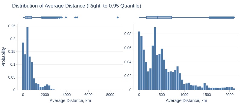
Key Observations:

• 75% of orders have seller-buyer distance ≤800km

• 5% ≤16.5km

• 5% ≥2,000km

• Several extreme outliers (>4,000km)

Let’s look by different dimensions.

By Whether the Order is Delayed or Not

pb.histogram(
    color='is_delayed'
    , upper_quantile=0.95
    , mode='dual_box_trim'
    , show_box=True
    , show_hist=False
    , show_kde=True
    , nbins=30
).show()
pb.bar_groupby(
    y='is_delayed'
    , to_slide=True
).show()

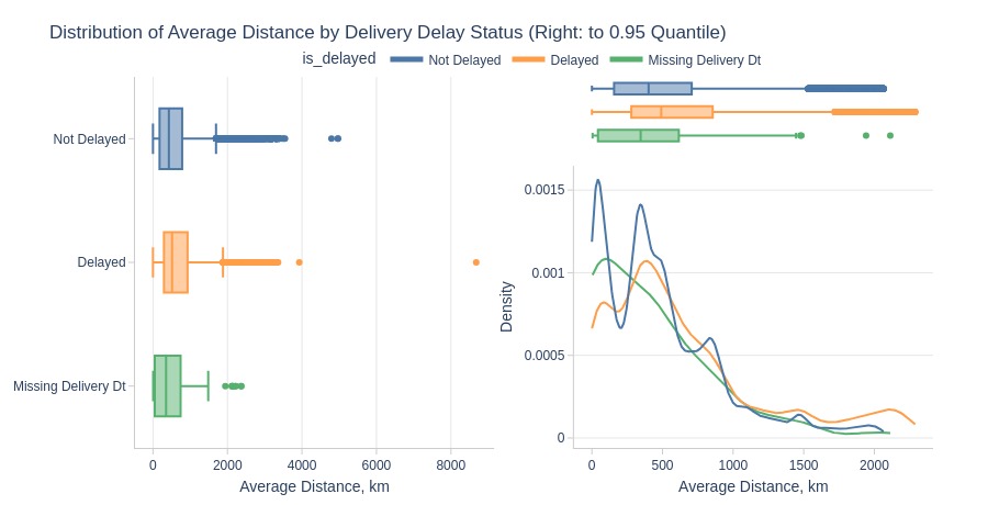
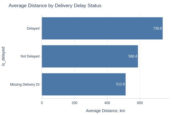
Key Observations:

• Delayed orders have greater average seller-buyer distance

By Presence of Installment Payments

pb.histogram(
    color='order_has_installment'
    , upper_quantile=0.95
    , mode='dual_box_trim'
    , show_box=True
    , show_hist=True
    , show_kde=False
    , nbins=30
).show()
pb.bar_groupby(
    y='order_has_installment'
    , show_count=True
    , to_slide=True
)

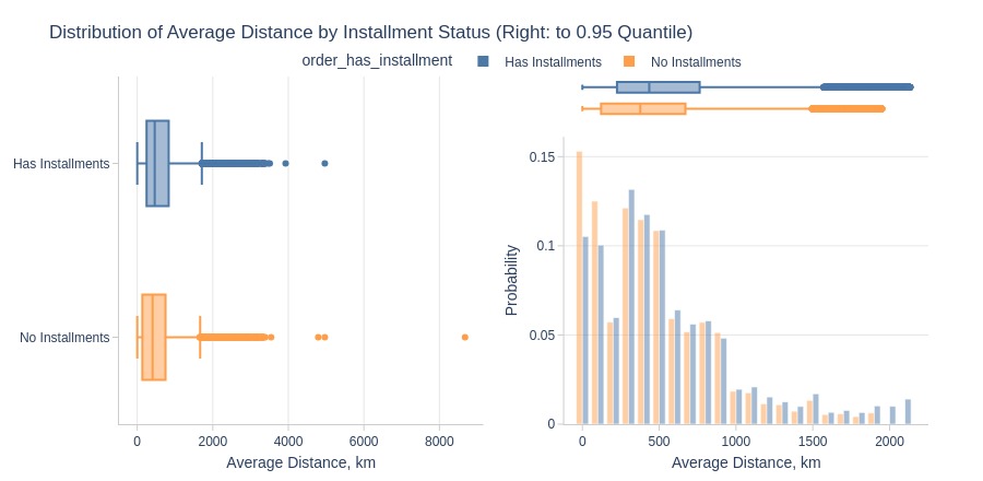
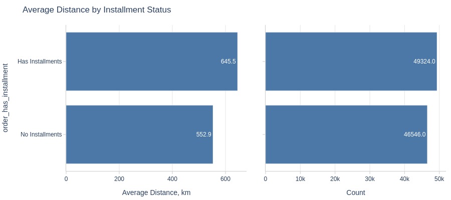
Key Observations:

• Installment orders have greater average seller-buyer distance

Delivery Time

Proportion of Each Stage in Delivery Time

Let’s look at what percentage of the total delivery time each stage occupies.

We will not consider any anomalous dates, as there are only a few and they will not significantly affect the result.

tmp_df_sales = (
    df_sales[[
        'order_purchase_dt',
        'order_approved_dt',
        'order_delivered_carrier_dt',
        'order_delivered_customer_dt',
    ]]
    [lambda x: (x.order_delivered_customer_dt >= x.order_purchase_dt) & (x.order_approved_dt >= x.order_purchase_dt)
        & (x.order_delivered_carrier_dt >= x.order_approved_dt) & (x.order_delivered_customer_dt >= x.order_delivered_carrier_dt)
     ]
    .dropna()
)

tmp_df_sales['from_purchase_to_customer'] = (tmp_df_sales['order_delivered_customer_dt'] - tmp_df_sales['order_purchase_dt']).dt.total_seconds()
tmp_df_sales['From Purchase to Approved'] = (
    (tmp_df_sales['order_approved_dt'] - tmp_df_sales['order_purchase_dt']).dt.total_seconds() * 100 / tmp_df_sales['from_purchase_to_customer']
).round(2)
tmp_df_sales['From Approved to Carrier'] = (
    (tmp_df_sales['order_delivered_carrier_dt'] - tmp_df_sales['order_approved_dt']).dt.total_seconds() * 100 / tmp_df_sales['from_purchase_to_customer']
).round(2)
tmp_df_sales['From Carrier to Customer'] = (
    (tmp_df_sales['order_delivered_customer_dt'] - tmp_df_sales['order_delivered_carrier_dt']).dt.total_seconds() * 100 / tmp_df_sales['from_purchase_to_customer']
).round(2) 

tmp_df_sales = (
    tmp_df_sales[['order_purchase_dt', 'From Purchase to Approved', 'From Approved to Carrier', 'From Carrier to Customer']]
    .melt(id_vars = 'order_purchase_dt', var_name='Stage', value_name='Percent of All Delivery Time')
    .rename(columns={'order_purchase_dt': 'Date'})
)

Let’s look at what percentage of the total delivery time each stage occupies on average.

sorted_means = tmp_df_sales.groupby('Stage')['Percent of All Delivery Time'].mean().sort_values(ascending=False)

annotations_data = [
    (0.6, -0.1, 'Carrier > Customer'),
    (-0.05, 0.8, 'Approved > Carrier'),
    (0.45, 1.08, 'Purchase > Approved')
]
fig = px.pie(
    values=sorted_means.values,
    names=sorted_means.index,
    title='Average Delivery Time Distribution by Stage',
    labels={'names': 'Delivery Stage', 'values': 'Percentage of Total Time'},
    category_orders={'names': ['From Carrier to Customer', 'From Approved to Carrier']},
    hole=0.4 
)
fig.update_traces(
    textinfo='percent',  
    textposition='inside', 
    texttemplate='%{percent:.1%}', 
    hovertemplate='%{label}: %{percent:.1%}', 
)
fig.update_layout(
    showlegend=False, 
    width=500,
    height=400,
    margin=dict(t=60),
    title_y=0.97
)
for x, y, text in annotations_data:
    fig.add_annotation(
        x=x,
        y=y,
        text=text,
        showarrow=False,
        font=dict(size=12)
    )
pb.to_slide(fig)
fig.show()

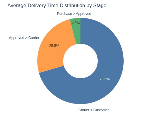
Key Observations:

• Delivery time distribution:

  • Payment approval: 4%

  • Carrier handoff: 25.5%

  • Carrier delivery: 70.5%

Look at distribution.

tmp_df_sales.viz.box(
    x='Percent of All Delivery Time'
    , y='Stage'
    , title='Percent of All Delivery Time by Stage'
)

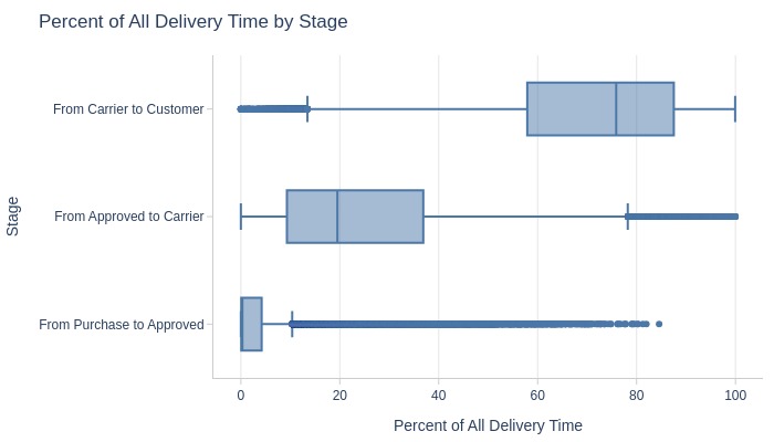
Key Observations:

• Carrier delivery consumes most of total delivery time

• Significant differences between stages (non-overlapping IQRs)

Total Delivery Time

pb.configure(
    df = df_sales
    , metric = 'delivery_time_days'
    , metric_label = 'Average Order Delivery Time, days'
    , metric_label_for_distribution = 'Order Delivery Time, days'
    , agg_func = 'mean'
    , title_base = 'Average Order Delivery Time and Number of Sales'
    , axis_sort_order='descending'
    , text_auto='.3s'
    , update_fig={'xaxis2': {'title_text': 'Number of Sales'}}
)

Top Orders

pb.metric_top()

	delivery_time_days
order_id
ca07593549f1816d26a572e06dc1eab6	209.63
1b3190b2dfa9d789e1f14c05b647a14a	208.35
440d0d17af552815d15a9e41abe49359	195.63
2fb597c2f772eca01b1f5c561bf6cc7b	194.85
285ab9426d6982034523a855f55a885e	194.63
0f4519c5f1c541ddec9f21b3bddd533a	194.05
47b40429ed8cce3aee9199792275433f	191.46
2fe324febf907e3ea3f2aa9650869fa5	189.86
2d7561026d542c8dbd8f0daeadf67a43	188.13
c27815f7e3dd0b926b58552628481575	187.74

Let’s see at statistics and distribution of the metric.

pb.metric_info(
    labels=dict(delivery_time_days='Order Delivery Time, days')
    , title='Distribution of Order Delivery Time'
    , upper_quantile=0.99
    , hist_mode='dual_hist_trim'
)

Summary Statistics for "delivery_time_days" (Type: Float)

Summary			Percentiles			Detailed Stats			Value Counts
Total	96.21k (99%)		Max	209.63		Mean	12.54		11.12	3 (<1%)
Missing	135 (<1%)		99%	46.01		Trimmed Mean (10%)	11.14		10.89	3 (<1%)
Distinct	93.55k (97%)		95%	29.21		Mode	Multiple		7.89	3 (<1%)
Non-Duplicate	90.94k (94%)		75%	15.68		Range	209.10		2.35	3 (<1%)
Duplicates	2.80k (3%)		50%	10.21		IQR	8.92		14.04	3 (<1%)
Dup. Values	2.60k (3%)		25%	6.76		Std	9.53		6.07	3 (<1%)
Zeros	---		5%	3.01		MAD	6.14		2.07	3 (<1%)
Negative	---		1%	1.82		Kurt	39.68		10.07	3 (<1%)
Memory Usage	1		Min	0.53		Skew	3.85		11.76	3 (<1%)

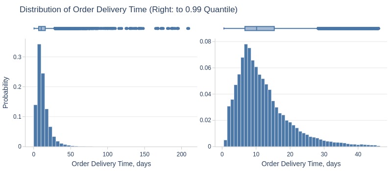
Key Observations:

• Median delivery time: ≥10 days

• 75% deliver in ≥16 days

• Top 5% take ≥30 days

Let’s look by different dimensions.

By Day of Week

pb.histogram(
    color='purchase_weekday'
    , upper_quantile=0.95
    , mode='dual_box_trim'
    , show_box=True
    , show_hist=False
    , show_kde=True
).show()
pb.bar_groupby(
    y='purchase_weekday'
    , show_count=True
).show()

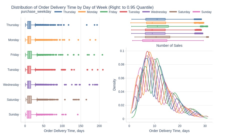
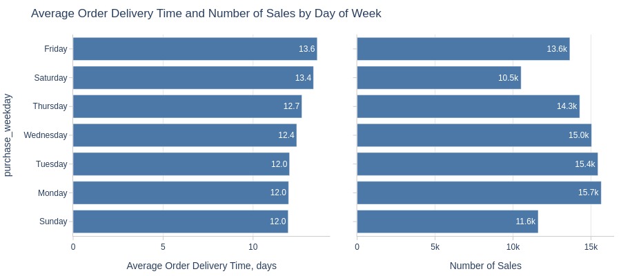
Key Observations:

• Friday/Saturday orders have slightly longer delivery times

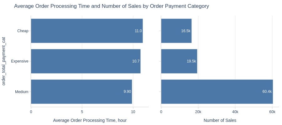
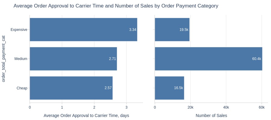
By Payment Category

pb.histogram(
    color='order_total_payment_cat'
    , upper_quantile=0.95
    , mode='dual_box_trim'
    , show_box=True
    , show_hist=False
    , show_kde=True
).show()
pb.bar_groupby(
    y='order_total_payment_cat'
    , show_count=True
    , to_slide=True
).show()

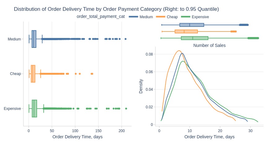
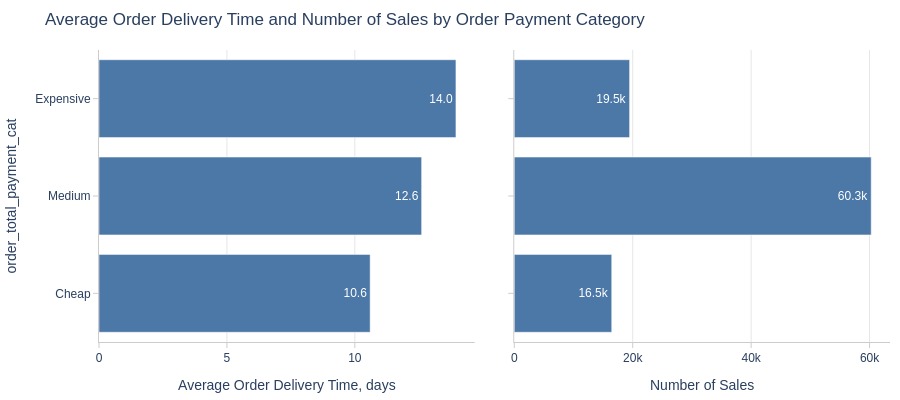
Key Observations:

• More expensive orders take longer to deliver

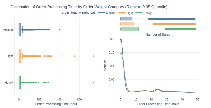
By Order Weight Category

pb.histogram(
    color='order_total_weight_cat'
    , upper_quantile=0.95
    , mode='dual_box_trim'
    , show_box=True
    , show_hist=False
    , show_kde=True
).show()
pb.bar_groupby(
    y='order_total_weight_cat'
    , show_count=True
    , to_slide=True
).show()

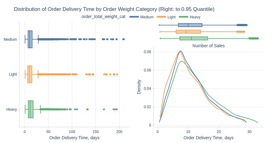
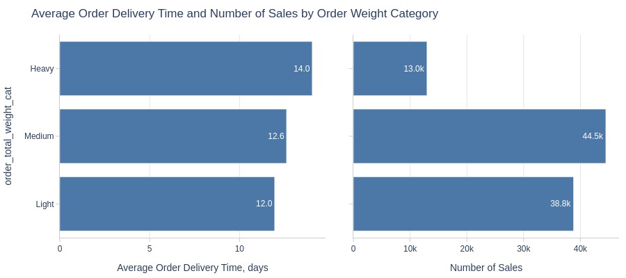
Key Observations:

• Heavy orders take longer to deliver than light/medium

By Review Score

pb.histogram(
    color='order_avg_reviews_score'
    , upper_quantile=0.95
    , mode='dual_box_trim'
    , show_box=True
    , show_hist=False
    , show_kde=True
).show()
pb.bar_groupby(
    y='order_avg_reviews_score'
    , show_count=True
    , to_slide=True
).show()

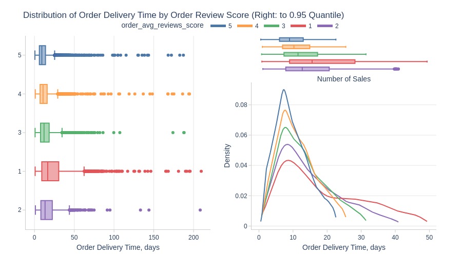
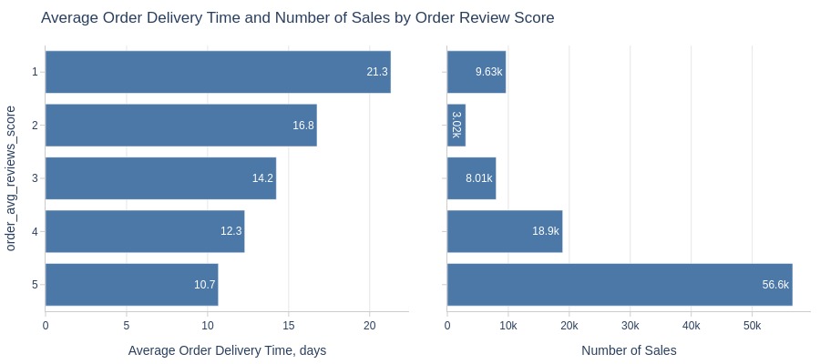
Key Observations:

• 1-star rated orders have noticeably longer delivery times

By Top Customer States

pb.box(
    y='customer_state'
    , upper_quantile=0.95
    , show_dual=True
).show()
pb.bar_groupby(
    y='customer_state'
    , show_count=True
    , to_slide=True
).show()

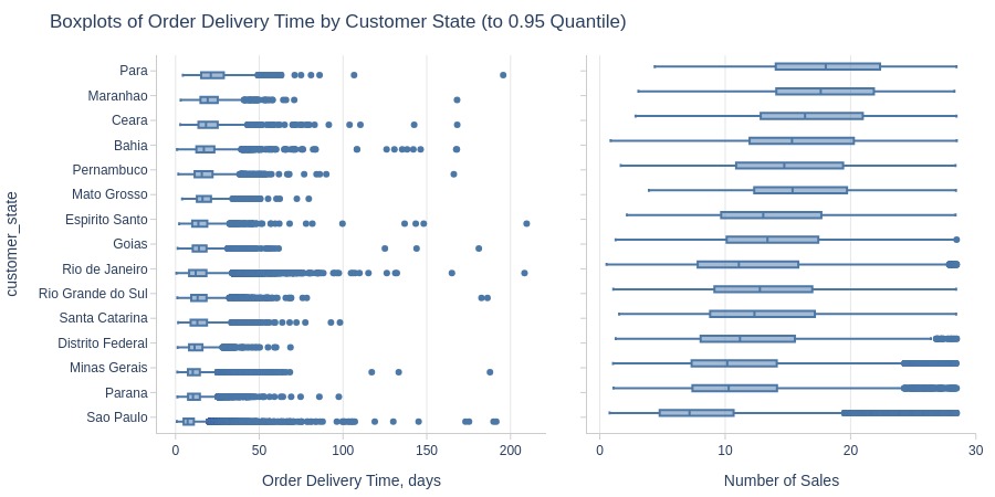
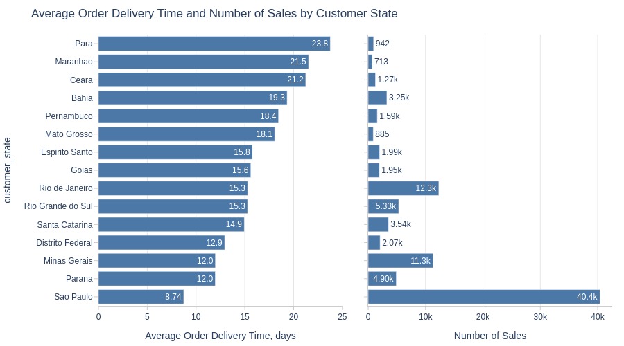
Key Observations:

• Among top states by sales volume, top 3 states with longest delivery times:

  1. Pará

  2. Maranhão

  3. Ceará

By Top Customer Cities

pb.box(
    y='customer_city'
    , upper_quantile=0.95
    , show_dual=True
).show()
pb.bar_groupby(
    y='customer_city'
    , show_count=True
    , to_slide=True
).show()

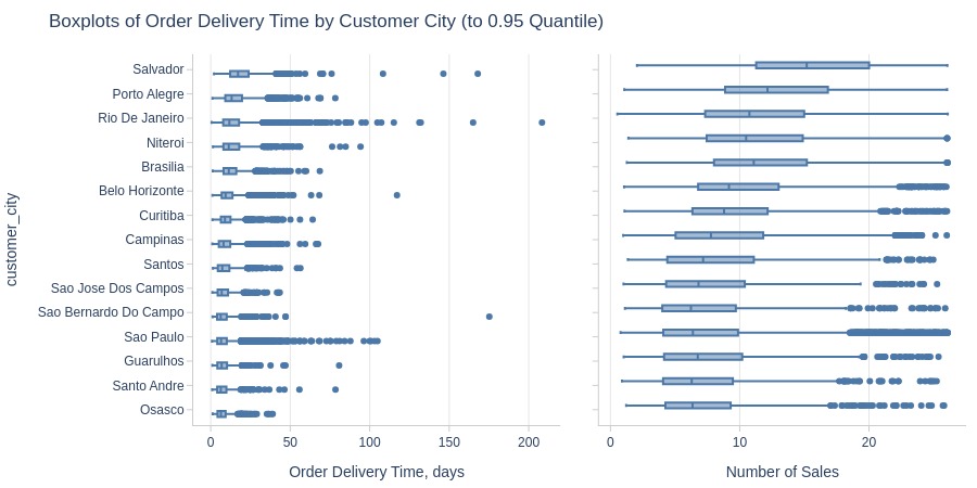
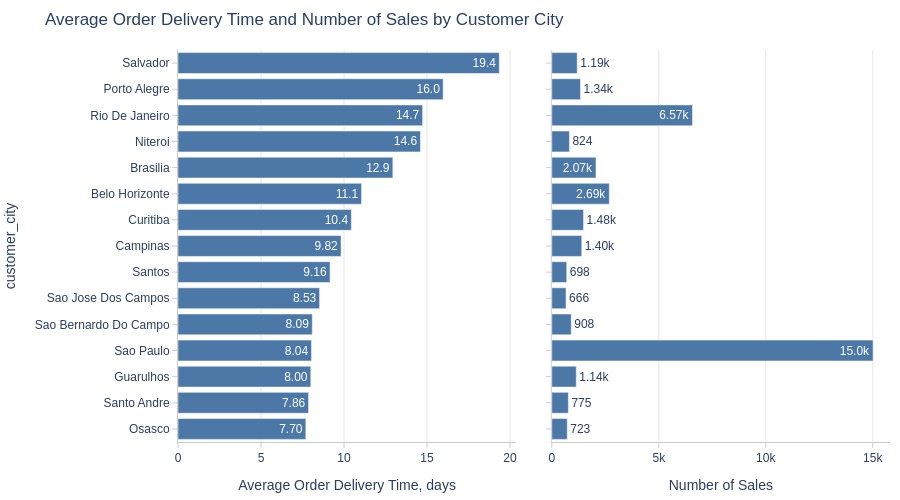
Key Observations:

• Among top cities by sales volume, top 3 cities with longest delivery times:

  1. Salvador

  2. Porto Alegre

  3. Rio de Janeiro

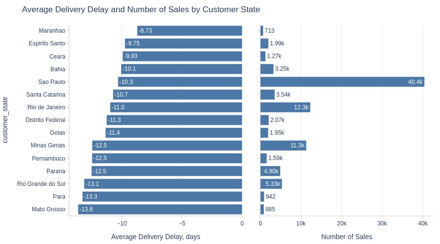
Delivery Delay

pb.configure(
    df = df_sales
    , metric = 'delivery_delay_days'
    , metric_label = 'Average Delivery Delay, days'
    , metric_label_for_distribution = 'Delivery Delay, days'
    , agg_func = 'mean'
    , title_base = 'Average Delivery Delay and Number of Sales'
    , axis_sort_order='descending'
    , text_auto='.3s'
    , update_fig={'xaxis2': {'title_text': 'Number of Sales'}}
)

Top Orders

pb.metric_top()

	delivery_delay_days
order_id
1b3190b2dfa9d789e1f14c05b647a14a	188.98
ca07593549f1816d26a572e06dc1eab6	181.61
47b40429ed8cce3aee9199792275433f	175.87
2fe324febf907e3ea3f2aa9650869fa5	167.71
285ab9426d6982034523a855f55a885e	166.58
440d0d17af552815d15a9e41abe49359	165.63
c27815f7e3dd0b926b58552628481575	162.72
d24e8541128cea179a11a65176e0a96f	161.78
0f4519c5f1c541ddec9f21b3bddd533a	161.61
2d7561026d542c8dbd8f0daeadf67a43	159.61

Let’s see at statistics and distribution of the metric.

pb.metric_info(
    labels=dict(delivery_time_days='Delivery Delay, days')
    , title='Distribution of Delivery Delay'
    , lower_quantile=0.01
    , upper_quantile=0.99
    , hist_mode='dual_hist_trim'
)

Summary Statistics for "delivery_delay_days" (Type: Float)

Summary			Percentiles			Detailed Stats			Value Counts
Total	96.21k (99%)		Max	188.98		Mean	-11.11		-12.39	5 (<1%)
Missing	135 (<1%)		99%	18.96		Trimmed Mean (10%)	-11.46		-13.28	4 (<1%)
Distinct	91.65k (95%)		95%	3.83		Mode	-12.39		-9.09	4 (<1%)
Non-Duplicate	87.39k (91%)		75%	-6.38		Range	334.99		-14.44	4 (<1%)
Duplicates	4.69k (5%)		50%	-11.82		IQR	9.84		-13.14	4 (<1%)
Dup. Values	4.26k (4%)		25%	-16.22		Std	10.09		-13.26	4 (<1%)
Zeros	---		5%	-25.37		MAD	7.02		-9.21	4 (<1%)
Negative	88.39k (92%)		1%	-34.31		Kurt	28.99		-15.08	4 (<1%)
Memory Usage	1		Min	-146.02		Skew	2.12		-7.22	4 (<1%)

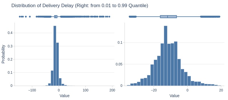
Key Observations:

• 75% of orders deliver ≥6 days early

• ~5% are ≥4 days late

By Review Score

pb.histogram(
    color='order_avg_reviews_score'
    , upper_quantile=0.95
    , mode='dual_box_trim'
    , show_box=True
    , show_hist=False
    , show_kde=True
).show()
pb.bar_groupby(
    y='order_avg_reviews_score'
    , show_count=True
    , to_slide=True
).show()

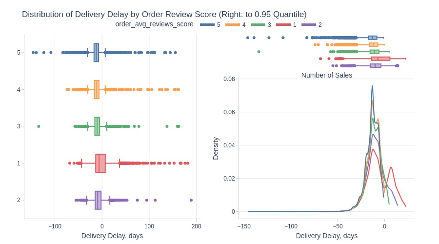
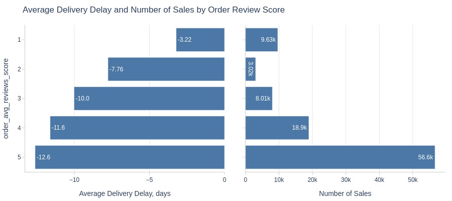
Key Observations:

• Higher rated orders deliver earlier than estimated

pb.box(
    y='customer_state'
    , upper_quantile=0.95
    , show_dual=True
).show()
pb.bar_groupby(
    y='customer_state'
    , show_count=True
    , to_slide=True
).show()

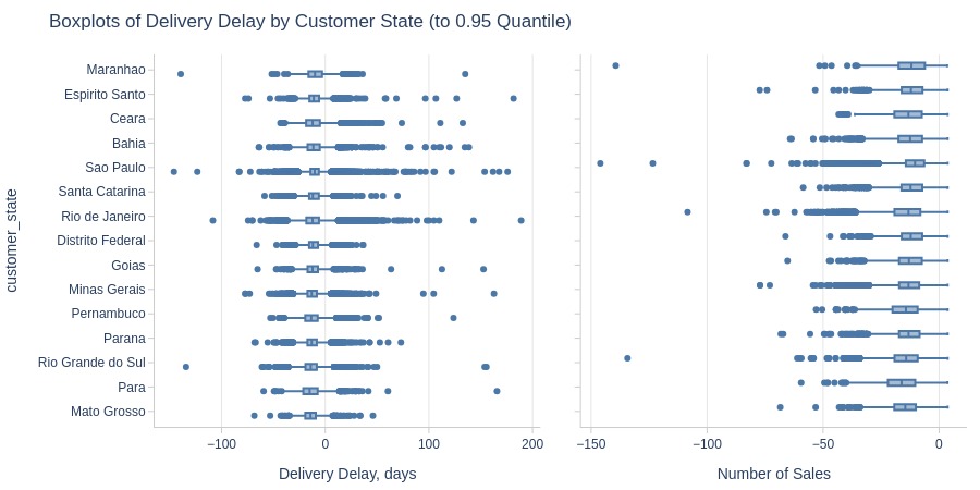
Key Observations:

• Among top states by sales volume, top 3 states for early delivery:

  1. Mato Grosso

  2. Pará

  3. Rio Grande do Sul

From Purchase to Approved Time

pb.configure(
    df = df_sales
    , metric = 'from_purchase_to_approved_hours'
    , metric_label = 'Average Order Processing Time, hour'
    , metric_label_for_distribution = 'Order Processing Time, hour'
    , agg_func = 'mean'
    , title_base = 'Average Order Processing Time and Number of Sales'
    , axis_sort_order='descending'
    , text_auto='.3s'
    , update_fig={'xaxis2': {'title_text': 'Number of Sales'}}
)

Top Orders

pb.metric_top()

	from_purchase_to_approved_hours
order_id
0a93b40850d3f4becf2f276666e01340	741.44
f7923db0430587601c2aef15ec4b8af4	738.45
de0076b42a023f53b398ce9ab0d9009c	554.78
daed0f3aefd193de33c31e21b16a3b3a	404.23
9c038e10f14d12a96939a0176c4ecc99	319.53
14ef2221cc3570aa6ce512fc353529b3	313.80
0c1426109d8295a688ee4182016bba59	300.43
483b53ea654d3566427a092cdef047fd	299.52
f5194ba2a4560ffa0e87746852c61fc1	298.94
70f357cca87c1162357bf3c0a993cbe5	291.41

Let’s see at statistics and distribution of the metric.

pb.metric_info(
    labels=dict(from_purchase_to_approved_hours='Order Processing Time, hour')
    , title='Distribution of Order Processing Time'
    , upper_quantile=0.99
    , hist_mode='dual_hist_trim'
)

Summary Statistics for "from_purchase_to_approved_hours" (Type: Float)

Summary			Percentiles			Detailed Stats			Value Counts
Total	96.35k (100%)		Max	741.44		Mean	10.25		0	1.24k (1%)
Missing	---		99%	89.69		Trimmed Mean (10%)	5.49		0.20	115 (<1%)
Distinct	32.51k (34%)		95%	48.20		Mode	0		0.19	113 (<1%)
Non-Duplicate	26.16k (27%)		75%	14.42		Range	741.44		0.19	112 (<1%)
Duplicates	63.83k (66%)		50%	0.34		IQR	14.21		0.20	109 (<1%)
Dup. Values	6.35k (7%)		25%	0.21		Std	20.51		0.21	109 (<1%)
Zeros	1.24k (1%)		5%	0.14		MAD	0.27		0.17	108 (<1%)
Negative	---		1%	0		Kurt	58.70		0.18	105 (<1%)
Memory Usage	1		Min	0		Skew	4.44		0.20	104 (<1%)

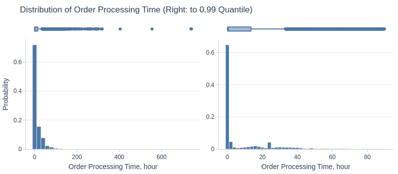
Key Observations:

• 75% of orders take ≥14 hours to process

• Top 5% take ≥48 hours

Let’s look by different dimensions.

By Day of Week

pb.histogram(
    color='purchase_weekday'
    , upper_quantile=0.95
    , mode='dual_box_trim'
    , show_box=True
    , show_hist=False
    , show_kde=True
).show()
pb.bar_groupby(
    y='purchase_weekday'
    , show_count=True
    , to_slide=True
).show()

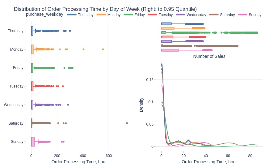
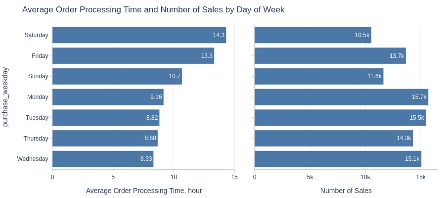
Key Observations:

• Friday/Saturday orders process slowest

• Wednesday orders process fastest

By Time of Day

pb.histogram(
    color='purchase_time_of_day'
    , upper_quantile=0.95
    , mode='dual_box_trim'
    , show_box=True
    , show_hist=False
    , show_kde=True
).show()
pb.bar_groupby(
    y='purchase_time_of_day'
    , show_count=True
    , to_slide=True
).show()

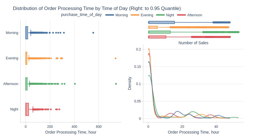
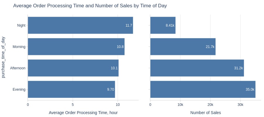
Key Observations:

• Nighttime orders take longer to process

By Whether the Order is Delayed

pb.histogram(
    color='is_delayed'
    , upper_quantile=0.95
    , mode='dual_box_trim'
    , show_box=True
    , show_hist=False
    , show_kde=True
).show()
pb.bar_groupby(
    y='is_delayed'
    , show_count=True
).show()

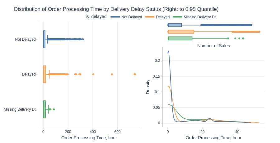
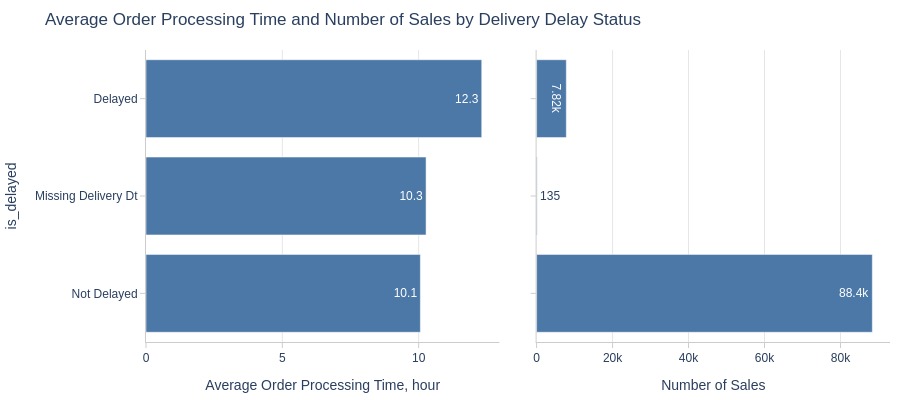
Key Observations:

• Non-delayed orders process faster (expected pattern)

By Weekday vs Weekend

pb.histogram(
    color='purchase_day_type'
    , upper_quantile=0.95
    , mode='dual_box_trim'
    , show_box=True
    , show_hist=False
    , show_kde=True
).show()
pb.bar_groupby(
    y='purchase_day_type'
    , show_count=True
    , to_slide=True
).show()

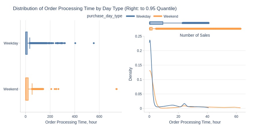
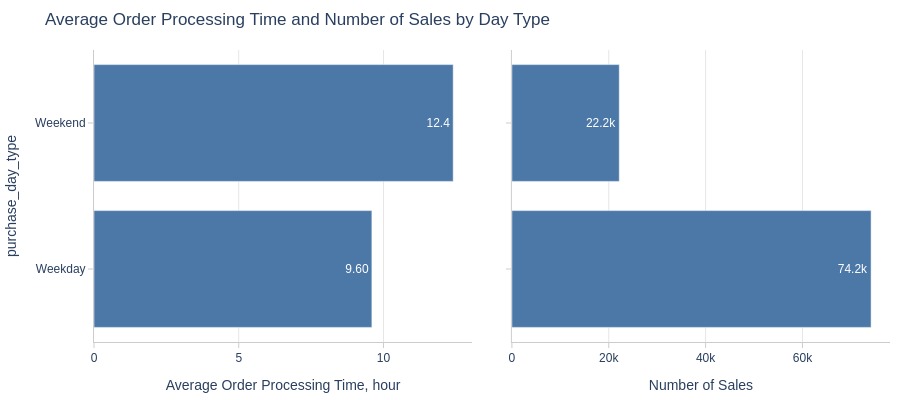
Key Observations:

• Weekday orders process significantly faster than weekends

By Payment Category

pb.histogram(
    color='order_total_payment_cat'
    , upper_quantile=0.95
    , mode='dual_box_trim'
    , show_box=True
    , show_hist=False
    , show_kde=True
).show()
pb.bar_groupby(
    y='order_total_payment_cat'
    , show_count=True
).show()

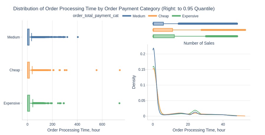
Key Observations:

• Cheap/expensive orders process faster than mid-priced

By Order Weight Category

pb.histogram(
    color='order_total_weight_cat'
    , upper_quantile=0.95
    , mode='dual_box_trim'
    , show_box=True
    , show_hist=False
    , show_kde=True
).show()
pb.bar_groupby(
    y='order_total_weight_cat'
    , show_count=True
).show()

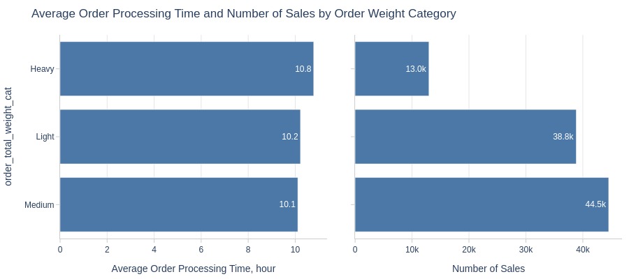
Key Observations:

• Heavy orders take longer to process

By Presence of Installment Payments

pb.histogram(
    color='order_has_installment'
    , upper_quantile=0.95
    , mode='dual_box_trim'
    , show_box=True
    , show_hist=False
    , show_kde=True
).show()
pb.bar_groupby(
    y='order_has_installment'
    , show_count=True
    , to_slide=True
).show()

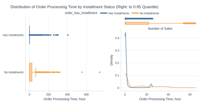
Key Observations:

• Installment orders process much faster

By Review Score

pb.histogram(
    color='order_avg_reviews_score'
    , upper_quantile=0.95
    , mode='dual_box_trim'
    , show_box=True
    , show_hist=False
    , show_kde=True
).show()
pb.bar_groupby(
    y='order_avg_reviews_score'
    , show_count=True
).show()

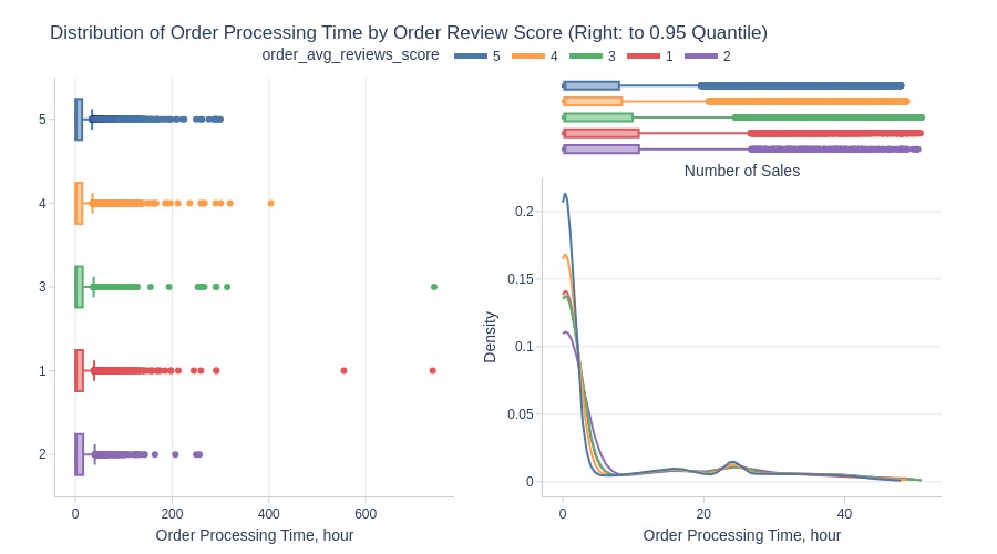
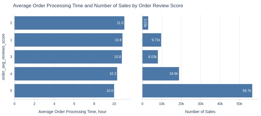
Key Observations:

• 1/2-star rated orders took longer to process

From Approval to Carrier Time

pb.configure(
    df = df_sales
    , metric = 'from_approved_to_carrier_days'
    , metric_label = 'Average Order Approval to Carrier Time, days'
    , metric_label_for_distribution = 'Order Approval to Carrier Time, days'
    , agg_func = 'mean'
    , title_base = 'Average Order Approval to Carrier Time and Number of Sales'
    , axis_sort_order='descending'
    , text_auto='.3s'
    , update_fig={'xaxis2': {'title_text': 'Number of Sales'}}
)

Top Orders

pb.metric_top()

	from_approved_to_carrier_days
order_id
da81fbc27b55e0f3d2813cf2078dc780	125.76
97f48024fcc76f1898e397ad6966e3a0	107.05
8b7fd198ad184563c231653673e75a7f	101.36
866314550f6d7a55c82917d9b4463e1f	64.57
a4a57f1ffa25b90dea9f150fee89db84	61.15
2805499c211b52dfc1e64a1349ef45e2	55.94
7d86c4aa9e59504b23f16c7ca68954a7	54.91
840d7cc10efae8ba460cc8ea84f1b6db	49.59
7141a7eee8944cb711fa1fd4f76300bc	49.34
bc9c2fb123725ad0d99fb76888543245	49.16

Let’s see at statistics and distribution of the metric.

pb.metric_info(
    labels=dict(from_approved_to_carrier_days='Order Approval to Carrier Time, days')
    , title='Distribution of Order Approval to Carrier Time'
    , upper_quantile=0.99
    , hist_mode='dual_hist_trim'
)

Summary Statistics for "from_approved_to_carrier_days" (Type: Float)

Summary			Percentiles			Detailed Stats			Value Counts
Total	96.31k (99%)		Max	125.76		Mean	2.81		1.85	1.35k (1%)
Missing	36 (<1%)		99%	16.56		Trimmed Mean (10%)	2.20		0.74	5 (<1%)
Distinct	85.11k (88%)		95%	7.99		Mode	1.85		0.94	5 (<1%)
Non-Duplicate	76.26k (79%)		75%	3.55		Range	125.76		0.82	5 (<1%)
Duplicates	11.23k (12%)		50%	1.85		IQR	2.64		0.91	5 (<1%)
Dup. Values	8.85k (9%)		25%	0.91		Std	3.38		0.88	4 (<1%)
Zeros	---		5%	0.32		MAD	1.64		0.79	4 (<1%)
Negative	---		1%	0.08		Kurt	65.14		2.21	4 (<1%)
Memory Usage	1		Min	0.00		Skew	5.14		0.93	4 (<1%)

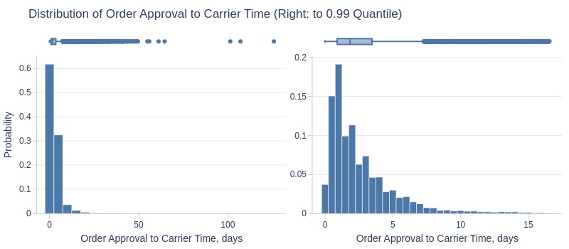
Key Observations:

• 75% of orders transfer to carrier within ≤3.5 days

• Top 5% take ≥8 days

Let’s look by different dimensions.

By Day of Week

pb.histogram(
    color='purchase_weekday'
    , upper_quantile=0.95
    , mode='dual_box_trim'
    , show_box=True
    , show_hist=False
    , show_kde=True
).show()
pb.bar_groupby(
    y='purchase_weekday'
    , show_count=True
    , to_slide=True
).show()

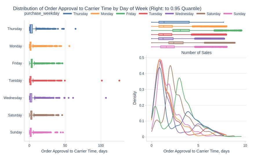
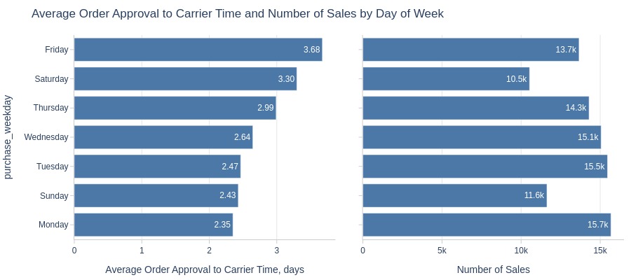
Key Observations:

• Friday/Saturday orders take longest to transfer to carrier

By Time of Day

pb.histogram(
    color='purchase_time_of_day'
    , upper_quantile=0.95
    , mode='dual_box_trim'
    , show_box=True
    , show_hist=False
    , show_kde=True
).show()
pb.bar_groupby(
    y='purchase_time_of_day'
    , show_count=True
).show()

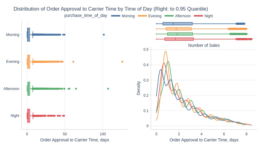
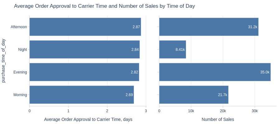
Key Observations:

• Morning orders transfer fastest to carrier

By Payment Category

pb.histogram(
    color='order_total_payment_cat'
    , upper_quantile=0.95
    , mode='dual_box_trim'
    , show_box=True
    , show_hist=False
    , show_kde=True
).show()
pb.bar_groupby(
    y='order_total_payment_cat'
    , show_count=True
    , to_slide=True
).show()

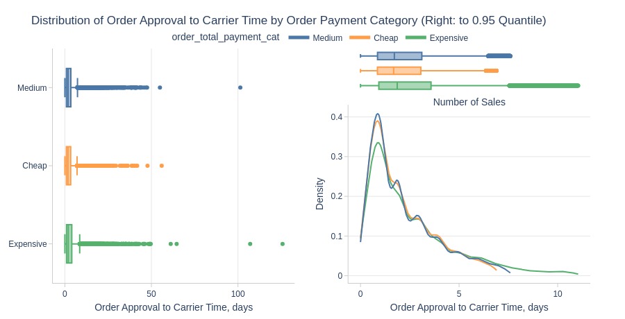
Key Observations:

• Expensive orders take longer to transfer to carrier

By Order Weight Category

pb.histogram(
    color='order_total_weight_cat'
    , upper_quantile=0.95
    , mode='dual_box_trim'
    , show_box=True
    , show_hist=False
    , show_kde=True
).show()
pb.bar_groupby(
    y='order_total_weight_cat'
    , show_count=True
    , to_slide=True
).show()

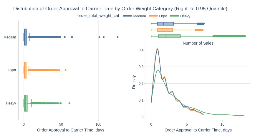
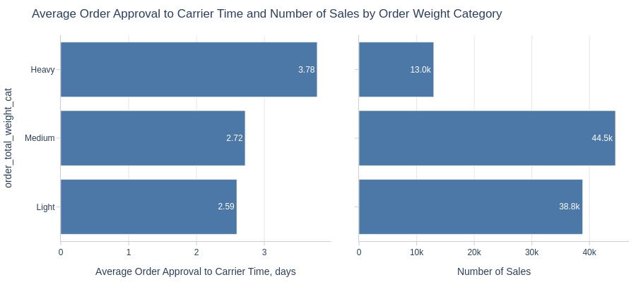
Key Observations:

• Heavy orders take longer to transfer to carrier

By Presence of Installment Payments

pb.histogram(
    color='order_has_installment'
    , upper_quantile=0.95
    , mode='dual_box_trim'
    , show_box=True
    , show_hist=False
    , show_kde=True
).show()
pb.bar_groupby(
    y='order_has_installment'
    , show_count=True
).show()

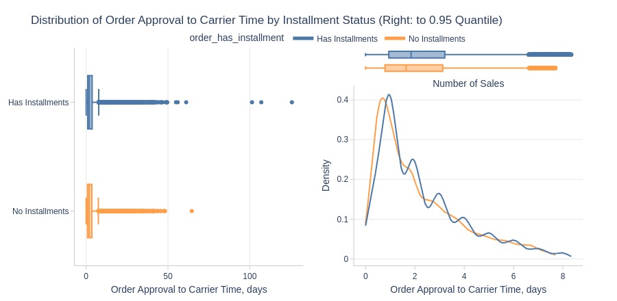
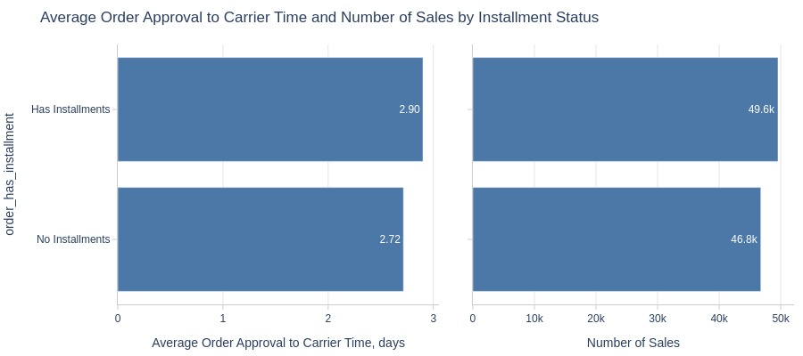
Key Observations:

• Installment orders take slightly longer to transfer to carrier

By Review Score

pb.histogram(
    color='order_avg_reviews_score'
    , upper_quantile=0.95
    , mode='dual_box_trim'
    , show_box=True
    , show_hist=False
    , show_kde=True
).show()
pb.bar_groupby(
    y='order_avg_reviews_score'
    , show_count=True
).show()

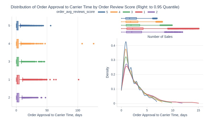
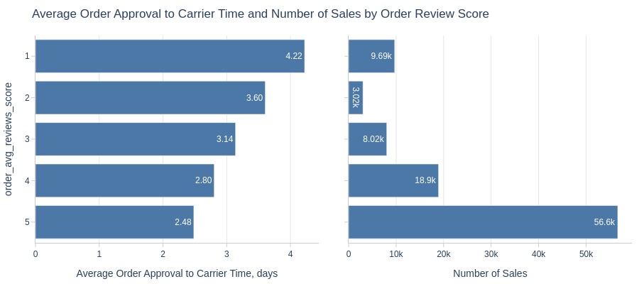
Key Observations:

• Faster carrier transfer correlates with higher ratings

Carrier Delivery Time

pb.configure(
    df = df_sales
    , metric = 'from_carrier_to_customer_days'
    , metric_label = 'Average Delivery Time from Carrier, days'
    , metric_label_for_distribution = 'Delivery Time from Carrier, days'
    , agg_func = 'mean'
    , title_base = 'Average Delivery Time from Carrier and Number of Sales'
    , axis_sort_order='descending'
    , text_auto='.3s'
    , update_fig={'xaxis2': {'title_text': 'Number of Sales'}}
)

Top Orders

pb.metric_top()

	from_carrier_to_customer_days
order_id
1b3190b2dfa9d789e1f14c05b647a14a	205.19
ca07593549f1816d26a572e06dc1eab6	195.03
285ab9426d6982034523a855f55a885e	194.21
2fb597c2f772eca01b1f5c561bf6cc7b	190.24
440d0d17af552815d15a9e41abe49359	188.09
2d7561026d542c8dbd8f0daeadf67a43	187.21
2fe324febf907e3ea3f2aa9650869fa5	186.40
437222e3fd1b07396f1d9ba8c15fba59	182.34
c27815f7e3dd0b926b58552628481575	182.10
dfe5f68118c2576143240b8d78e5940a	181.99

Let’s see at statistics and distribution of the metric.

pb.metric_info(
    labels=dict(from_carrier_to_customer_days='Delivery Time from Carrier, days')
    , title='Distribution of Delivery Time from Carrier'
    , upper_quantile=0.99
    , hist_mode='dual_hist_trim'
)

Summary Statistics for "from_carrier_to_customer_days" (Type: Float)

Summary			Percentiles			Detailed Stats			Value Counts
Total	96.21k (99%)		Max	205.19		Mean	9.34		7.10	20 (<1%)
Missing	135 (<1%)		99%	41.00		Trimmed Mean (10%)	7.97		0	8 (<1%)
Distinct	92.06k (96%)		95%	24.23		Mode	7.10		7.10	8 (<1%)
Non-Duplicate	88.10k (91%)		75%	12.04		Range	205.19		7.07	5 (<1%)
Duplicates	4.29k (4%)		50%	7.10		IQR	7.92		1.23	4 (<1%)
Dup. Values	3.96k (4%)		25%	4.11		Std	8.76		7.36	4 (<1%)
Zeros	8 (<1%)		5%	1.13		MAD	5.59		8.12	4 (<1%)
Negative	---		1%	0.82		Kurt	53.10		4.98	4 (<1%)
Memory Usage	1		Min	0		Skew	4.55		1.02	4 (<1%)

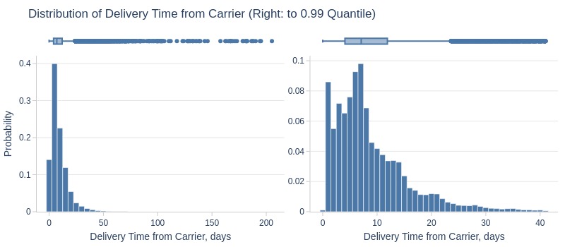
Key Observations:

• Median carrier delivery time: ≥7 days

• 25% take ≥12 days

• 5% take ≥24 days

Let’s look by different dimensions.

By Payment Category

pb.histogram(
    color='order_total_payment_cat'
    , upper_quantile=0.95
    , mode='dual_box_trim'
    , show_box=True
    , show_hist=False
    , show_kde=True
).show()
pb.bar_groupby(
    y='order_total_payment_cat'
    , show_count=True
    , to_slide=True
).show()

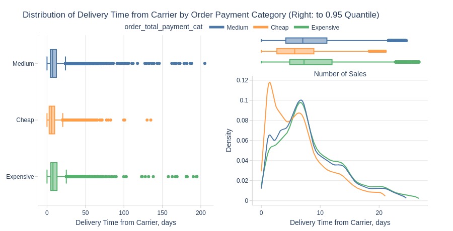
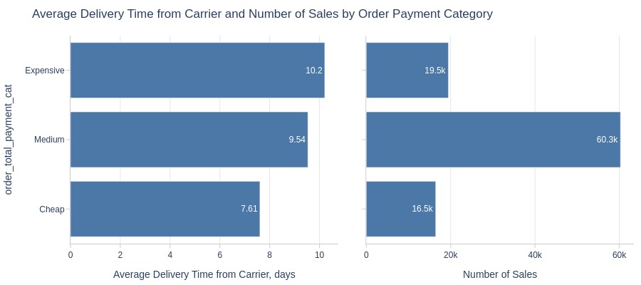
Key Observations:

• Cheap items deliver fastest via carrier

By Order Weight Category

pb.histogram(
    color='order_total_weight_cat'
    , upper_quantile=0.95
    , mode='dual_box_trim'
    , show_box=True
    , show_hist=False
    , show_kde=True
).show()
pb.bar_groupby(
    y='order_total_weight_cat'
    , show_count=True
).show()

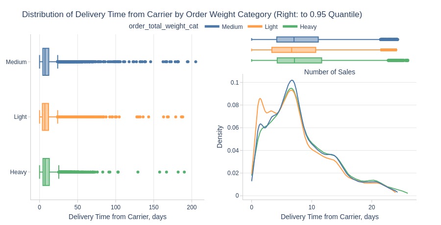
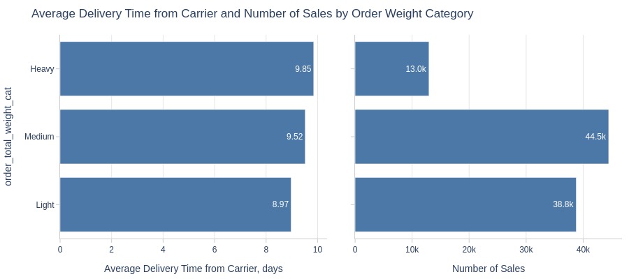
Key Observations:

• Light items deliver slightly faster via carrier

By Presence of Installment Payments

pb.histogram(
    color='order_has_installment'
    , upper_quantile=0.95
    , mode='dual_box_trim'
    , show_box=True
    , show_hist=False
    , show_kde=True
).show()
pb.bar_groupby(
    y='order_has_installment'
    , show_count=True
).show()

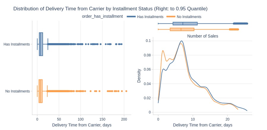
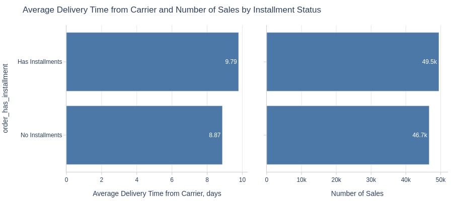
Key Observations:

• Installment orders take slightly longer via carrier

By Review Score

pb.histogram(
    color='order_avg_reviews_score'
    , upper_quantile=0.95
    , mode='dual_box_trim'
    , show_box=True
    , show_hist=False
    , show_kde=True
).show()
pb.bar_groupby(
    y='order_avg_reviews_score'
    , show_count=True
).show()

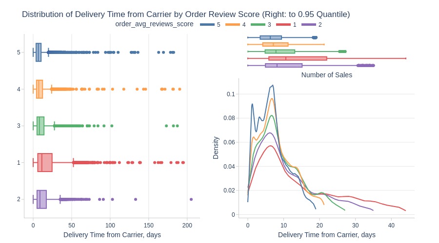
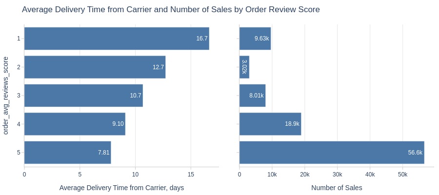
Key Observations:

• Longer carrier delivery times correlate with lower ratings

By Top Customer States

pb.box(
    y='customer_state'
    , upper_quantile=0.95
    , show_dual=True
).show()
pb.bar_groupby(
    y='customer_state'
    , show_count=True
    , to_slide=True
).show()

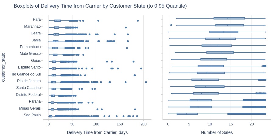
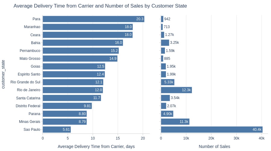
• Among top states by sales volume, top 3 states with longest carrier delivery:

  1. Pará

  2. Maranhão

  3. Ceará

By Top Customer Cities

pb.box(
    y='customer_city'
    , upper_quantile=0.95
    , show_dual=True
).show()
pb.bar_groupby(
    y='customer_city'
    , show_count=True
    , to_slide=True
).show()

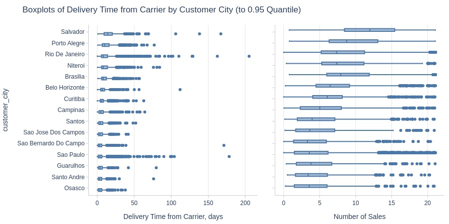
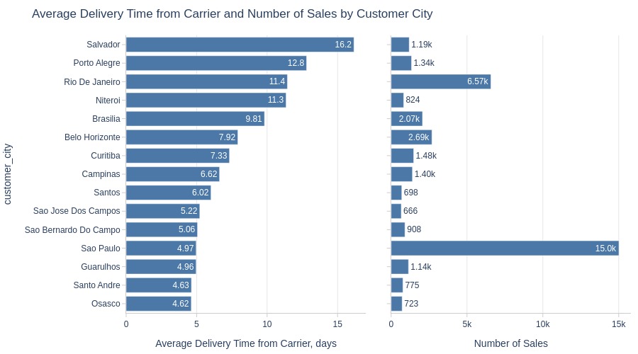
Key Observations:

• Among top cities by sales volume, top 3 cities with longest carrier delivery:

  1. Salvador

  2. Porto Alegre

  3. Rio de Janeiro

Carrier Handoff Delay

pb.configure(
    df = df_sales
    , metric = 'avg_carrier_delivery_delay_days'
    , metric_label = 'Average Carrier Delivery Delay, days'
    , metric_label_for_distribution = 'Carrier Delivery Delay, days'
    , agg_func = 'mean'
    , title_base = 'Average Carrier Delivery Delay and Number of Sales'
    , axis_sort_order='descending'
    , text_auto='.3s'
    , update_fig={'xaxis2': {'title_text': 'Number of Sales'}}
)

Top Orders

pb.metric_top()

	avg_carrier_delivery_delay_days
order_id
da81fbc27b55e0f3d2813cf2078dc780	116.76
8b7fd198ad184563c231653673e75a7f	95.36
97f48024fcc76f1898e397ad6966e3a0	91.05
866314550f6d7a55c82917d9b4463e1f	59.57
2805499c211b52dfc1e64a1349ef45e2	51.94
7d86c4aa9e59504b23f16c7ca68954a7	48.92
5d6e9993ecc20a59e637ce711858d081	45.91
abbbf52551bc34cd52a7851c06dfca90	45.43
d8734ba226623cf1c86b3cce8cbffa78	43.03
00e054d0da011d5016f31011af488f4f	42.90

Let’s see at statistics and distribution of the metric.

pb.metric_info(
    lower_quantile=0.01
    , upper_quantile=0.99
    , hist_mode='dual_hist_trim'    
)

Summary Statistics for "avg_carrier_delivery_delay_days" (Type: Float)

Summary			Percentiles			Detailed Stats			Value Counts
Total	96.31k (99%)		Max	116.76		Mean	-3.36		-1.14	4 (<1%)
Missing	36 (<1%)		99%	7.02		Trimmed Mean (10%)	-3.38		-5.70	4 (<1%)
Distinct	90.02k (93%)		95%	0.79		Mode	Multiple		-3.05	4 (<1%)
Non-Duplicate	84.06k (87%)		75%	-1.60		Range	1.16k		-5.03	4 (<1%)
Duplicates	6.33k (7%)		50%	-3.24		IQR	3.62		-2.18	4 (<1%)
Dup. Values	5.96k (6%)		25%	-5.22		Std	4.99		-2.96	4 (<1%)
Zeros	---		5%	-7.62		MAD	2.77		-1.77	4 (<1%)
Negative	87.72k (91%)		1%	-12.79		Kurt	19.89k		-5.45	4 (<1%)
Memory Usage	1		Min	-1.05k		Skew	-94.98		-5.04	4 (<1%)

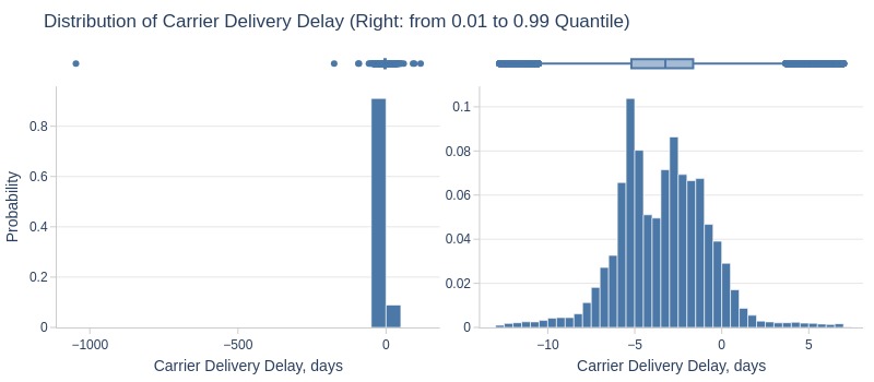
Key Observations:

• 75% of orders transfer to carrier ≥1.6 days early

• Extreme early transfers due to data anomalies

• 5% are ≥0.79 days late

• 1% are ≥7 days late

Let’s look by different dimensions.

By Review Score

pb.bar_groupby(
    y='order_avg_reviews_score'
    , show_count=True
).show()

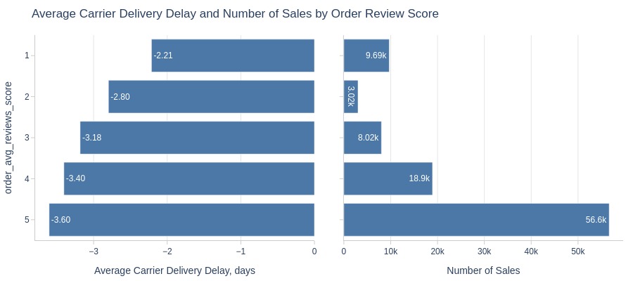
Key Observations:

• Earlier carrier transfer correlates with higher ratings